14.1 Skeletal currents and harmonic charts
The quantifier in the definition
Let have bidimension . A calibrated skeletal subset describes relative to a chart if for every smooth form tropicalized by and every compactly supported smooth scalar . In Definition 7.5.1, the current is skeletal when such a local description exists relative to every chart. The describing subset and calibration may depend on the chart.
This last quantifier is the essential point. Being supported on one skeleton only says where a current vanishes. Being skeletal specifies how it acts and how that action transforms when more tropical coordinates are introduced. The integration current of the ambient tropical space is skeletal because every chart has a canonically calibrated locus describing its top-dimensional integration.
Skeletal currents are symmetric and of order zero in the source construction. Positive describing calibrations give a correspondingly strong positivity statement. These conclusions come from their geometric description, independently of the false general implication from weak positivity to order zero discussed in Appendix A.
A simple example and a misleading near-example
On a weighted graph, integration over a collection of edges with constant compatible weights is a skeletal current. Multiplying by a nonconstant smooth scalar gives a current with the same support, but its edge density is no longer locally constant. It need not remain skeletal in this particular sense, and it need not remain closed. Thus support, order zero, skeletal representability, and closedness are four different properties.
Similarly, a Radon measure supported on a compact skeleton may have a singular continuous density or an arbitrary atomic distribution. It is a perfectly legitimate measure. It does not follow that it is a skeletal current of the required calibrated type. A theorem about the latter cannot be applied solely from the support of the former.
What harmonicity asks to vanish
The harmonic charts of CLD25 are built from the source’s PL-generated harmonic functions and current conditions. Their coordinates have vanishing appropriate Hessian currents, but their ordinary CLD smoothness is not assumed. Harmonicity is intended to preserve the integration and balancing needed for differential operations when the coordinate class is enlarged.
For a skeletal current, a coordinate interacts with the calibration through . If this vanishes, the weighted slopes of cancel in the relevant skeletal description. This is a stronger compatibility with than merely on the ambient integration current. That difference is exactly why the Bedford–Taylor property later appears in the harmonic product theorem.
The mechanism of the harmonic product formula
Proposition 8.11.1 assumes that is skeletal and has the Bedford–Taylor property. For a G-form locally obtained from harmonic coordinates, it proves the expected differential identities The proof applies Stokes to the skeletal pieces. The internal boundary terms involve the outgoing derivatives of the harmonic coordinate functions. The Bedford–Taylor property turns their ambient Hessian vanishing into , which forces the required weighted cancellation. Thus the hypothesis has a concrete job: it makes the new coordinates harmonic for the current being multiplied.
Corollary 8.11.2 then identifies certain recursively defined BT products with products by the corresponding G-forms. Its skeletal and BT hypotheses are retained here. The subsequent Corollary 8.11.3 is stated for an arbitrary positive closed current but cites this restricted comparison. Section 14.2 gives an explicit counterexample in the abstract tropical category. The restricted theorem cannot be extended by simply dropping those hypotheses.
14.2 The kernel problem: a complete tropical calculation
The equality one wants to descend
For an admitted continuous potential and a positive closed current , the expression is defined. To say that it depends only on asks for for differences of admitted potentials. This is a statement about the kernel of the ambient Hessian acting on . It does not follow from approximation independence, which says that two approximating sequences for the same function give the same product.
For smooth , closedness of gives , so the implication holds. For a smooth analytic-unit logarithm, this proves exactly the gluing needed for line-bundle weights. For a nonsmooth current-harmonic , the same Leibniz proof is not available.
An admissible reducible tropical space
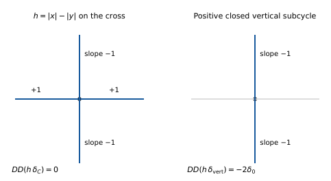
Let , , and . Give each of the four rays weight one. Use the refined affine structure of CLD25 Example 6.1.4: affine functions are locally restrictions of ambient affine functions on . In particular, not every PL function is declared affine.
Here are the category checks, since the example is meant to test an abstract tropical theorem. The underlying polyhedral structure has the G-tropical and skeletal structures of Examples 5.1.4 and 5.2.3. It is pure of dimension one and has the required richness. Ambient coordinates separate points and differential directions. An affine germ on a polyhedral domain extends from its ambient affine expression, and such domains are locally Boolean combinations of affine inequalities; these give the two decency conditions in Definition 6.3.1. The calibration balances at the vertex because Every local affine chart preserves this equation. Boundaries of local polyhedral domains have zero one-dimensional measure. Thus Definition 6.6.2 permits the empty boundary. The larger boundary allowed as a general choice in Example 6.6.3 does not force the vertex to be a boundary point in this balanced example.
Smooth tests for this structure are locally restrictions of ambient smooth superforms. In particular, their restrictions to each whole line are smooth through the origin, and scalar tests have one common value at the vertex.
Two potentials with the same ambient curvature
Put and . The restrictions of are smooth psh functions decreasing uniformly to as . Thus both belong to the one-stage continuous approximation class. For every smooth compactly supported scalar test , Hence on the same actual test space.
Now let , integration of -tests along the horizontal line. This is a positive current, and Stokes on the whole line proves . Multiplication by the continuous functions gives The current is therefore positive closed but fails the BT kernel property. All identities use the same tests; no tensor-product-only testing or change of category is hidden in the calculation.
The consequence for harmonic pullback
The function is PL and satisfies . It is harmonic by CLD25 Definition 7.8.2. Take the harmonic map and the convex function . Then is a difference of the admitted psh potentials, but This is not positive. Thus Corollary 8.11.3 is false in its unrestricted abstract-tropical formulation. The missing skeletal/BT hypothesis in its cited argument is not merely cosmetic. This calculation strengthens the hypothesis-transfer observation in the preceding audit section to a counterexample in the explicitly verified category.
The example does not satisfy the hypotheses of a smooth Berkovich local-potential problem. It does not refute a separate analytic theorem based on residual geometry. Its conclusion is confined to the stated abstract tropical generality.
The graph-support statement also detects the problem
On , with coordinate in the second factor, put and use . The graph-intersection construction of §9.5 is On the open set we have . Hence is disjoint from , but the restriction of the displayed current to is which is nonzero. Indeed, take a test supported in , with and nonzero. Its pairing is .
This disproves the unrestricted harmonic graph-support assertion in Lemma 9.5.4. Its printed proof uses a BT hypothesis on that is not in the statement. For an affine , the relevant potential is smooth affine off the graph and the closed-current Leibniz calculation does prove the support assertion. A version with additional BT hypotheses must verify the corresponding stability and potential class.
What remains a valid research question
The cross shows that arbitrary-current kernel descent cannot be proved from the abstract tropical axioms alone. A positive answer on a smooth analytic space must use extra analytic geometry or a more restrictive harmonic kernel. Possible inputs include residual numerical triviality, approximation preserving the relevant kernel, or a representation theorem for the allowed currents. Finding such an input is a substantive theorem, not a change of notation.
References. [CLD25] (Examples 5.1.4, 5.2.3, 6.1.4; Definitions 6.3.1, 6.6.2, 7.8.2; Corollary 8.11.3 and Lemma 9.5.4).
14.3 A local classification of the graph kernel property
The tropical cross gives a counterexample, but its mechanism is more general. On a balanced graph, the ambient Laplacian and the Laplacian weighted by another current are two linear functionals on the vector of outgoing slopes. Potential independence asks for inclusion of their kernels. This elementary linear-algebra problem can be solved completely.
Let a neighbourhood of a vertex be a union of rational rays with primitive outgoing vectors , parameterized by lattice length . Give them positive weights satisfying . Smooth tests are restrictions of ambient smooth superforms. Let be integration along the same rays with nonnegative constant weights . We work with compactly supported tests in this neighbourhood, so artificial outer endpoints contribute no boundary terms.
NAG-900278 Proof review pending
Lemma 14.3.1. The current is closed under both and if and only if . If this balancing condition holds and a continuous function is affine on each ray near , with outgoing slopes , then its vertex contribution is
Proof. Stokes on each ray expresses the boundary of its integration current as evaluation at against the outgoing tangent. Summing with weights gives contraction with . Thus balancing is sufficient. Conversely, choose an ambient covector and a smooth cutoff equal to one near . The associated one-form test detects . Vanishing for every forces balancing. The two differentials give the same condition in their respective exterior factors.
For the second assertion, write . Twice integrating by parts against a scalar test gives the vertex terms . The terms containing sum to zero by balancing. The remaining sum is the displayed atom. There is no interior term because each is affine near the vertex. ◻
NAG-900279 Proof review pending
Theorem 14.3.2. Assume is closed. The following conditions are equivalent:
For every continuous, raywise affine germ at , ambient harmonicity implies near .
There is a constant such that for every .
Thus, in this class of currents and PL germs, the full ambient harmonic kernel acts trivially precisely when the current has a common density relative to the ambient calibration.
Proof. Any vector is realized by a continuous raywise affine germ with a prescribed common value at . By Lemma 14.3.1, condition (1) is therefore Fix an index . Since , every decomposes as with the first term in . Kernel inclusion gives for all , so with . Conversely, proportionality gives , proving (1). It also automatically gives balancing from that of . ◻
The theorem concerns all continuous raywise affine germs. If a particular analytic theory admits a smaller harmonic class, its kernel condition can be weaker. In particular, the theorem does not assert that every such germ on every graph is the restriction of an analytic harmonic function. That realization problem involves the analytic or residual geometry absent from this linear-algebra calculation.
NAG-900280 Proof review pending
Corollary 14.3.3. Let a connected finite balanced graph have positive ambient edge weights, and let a closed polyhedral integration current have constant nonnegative weights on its edges. If the local property of Theorem 14.3.2 holds at every vertex, then the current is one constant nonnegative multiple of the ambient integration current.
Proof. At a vertex, the theorem says that the ratios of current weight to ambient weight are the same on all incident edges. An edge has one ratio at both ends because both of its weights are constant. Connectedness propagates the ratio through the graph. The statement is componentwise if the graph is disconnected. ◻
Why ordinary closedness is weaker
An ambient affine function has slopes . Closedness gives . Thus closedness already annihilates all slopes coming from ambient affine functions. The harmonic kernel usually contains more slopes: it is the hyperplane , whereas the affine slopes form the image of . Equality of these two spaces requires an additional rank condition.
Example 14.3.4. For the standard trivalent tropical line, , and . Balancing forces . With ambient weights one, every closed current in this constant-edge class therefore satisfies the PL kernel property.
For the cross, the directions are . Balancing only forces weights of the form . Theorem 14.3.2 requires . The slopes are ambient harmonic and give weighted Laplacian . Taking , recovers the earlier counterexample. The failure is measured by the difference between the densities on the two crossing lines.
This calculation explains the role of an extra BT property in a harmonic-coordinate theorem. Such a property is a compatibility requirement between the allowed harmonic functions and the current’s calibration. It is not another name for positivity and closedness. In a Berkovich theorem, proving that compatibility may require residual geometry or a representation theorem; it cannot be replaced by the smooth Leibniz rule for coordinates which are not smooth in the original sheaf.
14.4 The obstruction to gluing local potentials
A local potential theorem and a global potential theorem are different assertions even on a smooth real affine manifold. Local potentials differ by elements of the Hessian kernel. Their differences form a cocycle, and this cocycle is the exact obstruction to choosing one global potential. This elementary description is useful when comparing Green currents, metric weights and cohomological vanishing.
Let be a paracompact real affine manifold, with affine transition maps, and let be the sheaf of locally affine real functions. On convex coordinate charts, Theorem 11.5.3 gives convex potentials for any ordinary positive closed current. Affine coordinate changes preserve Hessians and convexity. Choose a cover by such charts and potentials .
NAG-900281 Proof review pending
Proposition 14.4.1. On every overlap, is locally affine, and The resulting class in is independent of the local potentials and cover. It vanishes if and only if the current is the Hessian of a global finite locally convex function.
Proof. The difference has zero Hessian, hence is affine on each connected overlap component by Proposition 11.4.1. The cocycle identity is subtraction of three functions. If is replaced by another potential, its difference from the old one is a locally affine function , and the new cocycle differs by . Refinement restricts the same cocycle. Thus the class is intrinsic.
If the class vanishes, after refinement there are locally affine with . Then agree on overlaps and glue to a finite continuous function . Locally it is convex and has the prescribed Hessian. Conversely, a global potential gives and makes the cocycle a coboundary. ◻
The coefficient sheaf is , not the constant sheaf . On a singular tropical space, the kernel of the Hessian current can differ from the restrictions of affine functions. Replacing that kernel by an ambient affine sheaf would change the obstruction group. The tropical cross in Chapter 14 gives an explicit reason for retaining the actual kernel.
Example 14.4.2. (A positive curvature class on a real torus). Let , and let be a positive definite symmetric matrix. The form descends to . Locally it is for . On overlaps of lifted charts differing by , This is an affine cocycle. It cannot be a coboundary of local affine functions, because a global distributional potential would give a contradiction. The first equality is distributional integration by parts and . Thus a perfectly regular positive curvature form can have local convex potentials and no global scalar potential.
Metric weights solve a different gluing problem
For a line bundle with local frames and transitions , additive metric weights satisfy The transition functions are prescribed by the line bundle. Their logarithms are smooth pluriharmonic where are analytic units, so the local currents glue even when the weights do not glue as scalar functions. A metrized line bundle is therefore naturally described by local potentials with a specified cocycle. The global scalar-potential problem asks for that cocycle to be trivial in the relevant kernel sheaf.
This also explains a limitation of curvature comparison. Equal local curvatures imply that the difference of weights lies in a Hessian kernel. They do not identify the metric constants or the transition cocycle without further information. In the real affine case the kernel is fully described above; in a non-Archimedean form theory its description depends on the chosen tests and regularity class.
References. The local real potential theorem is [Lag12] (Proposition 1.13). The cocycle argument is the standard gluing construction applied to its affine kernel; the torus automorphy formula is compatible with the metric setting of [BGJK25] (Sections 7–8).