Chapter 4 constructed the annular and semistable curve skeleta. We use them here to compare tropical maps, integral lattice indices and canonical analytic lifts. Section 3.8 supplies the residue-dimension calculation for the higher-dimensional local model.
6.1 Skeleta and tropical images
The Gauss section of a torus
For , define a weighted Gauss norm on the Laurent algebra by It is a multiplicative norm and therefore a point of . The minus sign in the exponential is forced by . In particular, The set is the torus skeleton. The map is continuous and identifies with this subset of ; a separate deformation-retraction theorem makes a strong deformation retraction. Having a section alone would not prove that theorem.
Equation (6.1.1) also gives the exact identity The Gauss norm retains the largest size among the terms, even when several sizes agree. It does not perform the cancellation that can occur at other points in the same tropical fibre.
References. [GRW16] (Sections 3–4); Proposition 5.5.1.
Example 6.1.1. (The ambient section misses the hypersurface). Let . For every , Thus , including when . A point of must annihilate its defining equation. The ambient Gauss point does not.
Consequently, restricting to does not produce a section . A section for a subvariety, when a theorem supplies one, must choose different analytic points. Likewise, the ambient torus deformation retraction need not preserve .
This elementary example is a useful safeguard. The tropicalization is a subset of a real vector space; a skeleton is a subset of an analytic space. A map can identify suitable pieces of them, but the identification is additional structure or an additional theorem.
Annuli, lengths, and integral slopes
The annular skeleton and its retraction were constructed in Section 4.3 and illustrated in Figure 4.1. Its coordinate has integral slope one. We now compare the logarithmic metric with lattice indices and model multiplicities.
For the local semistable equation , with , the annular skeleton has coordinate and interval If over a discretely valued field, its length is , where . It becomes only after the explicit normalization .
For a curve with a chosen semistable model, annular pieces assemble into a metric graph. Over a non-algebraically-closed residue field, residual degrees can contribute weights to its slope formulas. The model, the graph, its metric, and these weights must all be specified. A smallest skeleton need not contain enough cells to represent every differential form: a curve with good reduction can have a one-point minimal skeleton, although its local differential calculus is not zero.
There are also several kinds of boundary. The endpoints of a closed annulus belong to its analytic boundary, whereas an open annulus is boundaryless. A facet in a chosen polyhedral subdivision is a combinatorial notion. A component removed from an algebraic compactification is yet another notion. Balancing away from an analytic boundary cannot be silently applied at the endpoint of a restricted annulus.
References. [GRW16] (Sections 3–4 and 9–10).
For a discretely valued field with uniformizer , write . The annulus has length . Its integral slope for the function is one, while the change in function value is . The integer , the real length, and the slope are different quantities. If an algebraic intersection length is , the associated logarithmic height has the factor in this normalization. By contrast, the total mass of the Chern measure of a degree-one model line is one.
Example 6.1.2. (Power maps on annuli). Let and . The map takes to . If , the target skeletal coordinate is . Thus the target interval has times the source length, and the image of the source integral tangent lattice has index in the target lattice. The map is finite of degree : the equation is monic and the source algebra is free of rank over the target algebra. This includes the inseparable case. The integral slope and algebraic degree retain the multiplicity that a count of distinct fibres can miss.
A semistable local model and its simplex
Over a discretely valued field, a basic strictly semistable model has an tale local chart Write . Its skeleton is locally described by This is an -simplex. Its dimension is , while the generic fibre has dimension . The remaining coordinates describe directions not recorded by this simplex.
On the special fibre, the equation becomes : the components are the coordinate hyperplanes. Their intersections are normal-crossing strata. For the transversal picture is a node; for larger , several components meet normally. These semistable equations control the singularities of the special fibre. Over a general valuation ring we do not additionally assert that the underlying formal model is a noetherian regular scheme. A stratum where more components meet corresponds to a simplex of higher dimension. Thus a skeleton records incidence and valuation data, not every residual algebraic direction.
Faithful tropicalization and multiplicity-one sections
In this subsection, let be complete, algebraically closed, and nontrivially valued. Let be a strictly semistable pair in the proper algebraic setting of Gubler–Rabinoff–Werner. Its skeleton lies in the analytic generic fibre, with unbounded directions when the horizontal divisor is present. A tropicalization is faithful on this skeleton if it is injective there and unimodular on its polyhedral pieces: it preserves the integral tangent lattices, not just the topology.
NAG-900024 Proof review pending
Theorem 6.1.3. (GRW, Theorem 9.5). In the strictly semistable-pair setting of [GRW16], there exists a finite collection of nonzero rational functions on the generic fibre whose tropicalization is faithful on .
The rational functions are regular units on a suitable dense open containing the relevant skeletal points. The assertion does not say that every preassigned moment map is faithful. Nor does it say that the entire analytic space is homeomorphic to the skeleton. The added rational functions can have divisors outside ; the resulting tropicalization need not factor through the skeletal retraction [GRW16] (Remark 9.6).
A different theorem starts with an embedding of a very affine integral variety into a torus. On a subset of its tropicalization where the tropical multiplicity is one, each tropical fibre has a unique Shilov boundary point. These points give a continuous partial section . If is contained in the closure of its interior in the whole tropicalization, this is the unique continuous section on [GRW16] (Theorem 10.6). This statement concerns multiplicity-one fibres, and is not obtained by restricting the ambient torus Gauss section.
On a curve with good reduction, a natural compact skeleton may consist of one point. If all differential forms factored through that point, every positive-degree form would vanish. Local annular and punctured-disc domains still admit nonconstant tropical coordinates and nonzero forms. Therefore global factorization through a chosen small skeleton is a property of special data, not a general consequence of the existence of a skeleton.
Payne’s inverse limit: what is recovered
For a quasiprojective variety over a complete algebraically closed nontrivially valued field, Payne identifies its analytification with the inverse limit of extended tropicalizations over the appropriate system of toric embeddings: This is a homeomorphism of topological spaces [Pay09] (Theorem 4.2). The transition maps remember how a larger collection of characters projects to a smaller one.
The reason a whole system is needed can already be seen in one tropical fibre. A fixed tuple of values may be shared by many analytic points. Adding more functions can distinguish them. The inverse limit requires compatible values for all such choices and recovers the seminorm, whereas one finite tropicalization records only part of it.
There are three different questions here:
| Question | Additional structure needed |
|---|---|
| Recover the underlying topology | The inverse system of extended tropicalizations. |
| Recover analytic functions and their norms | Analytic or formal models and compatible sheaves; a bare topological homeomorphism is insufficient. |
| Recover forms, currents, and their operations | Test spaces, quotient relations, refinements, and continuity of the operations. |
A smooth form has locally finite tropical presentations by definition. This fact is not a consequence that every current factors through one finite tropicalization. Likewise, a Hodge theorem on selected tropical spaces does not automatically pass through this inverse limit: the relevant complexes, transition maps, cohomology, and exactness must first be compared.
6.2 Fans and extended tropicalization: keeping the boundary
Cones specify which limits are admitted
A torus excludes the zero and pole loci of its characters. This is convenient locally, but a projective variety cannot in general be embedded in one torus. To describe a compactification, tropical geometry must allow some character valuations to tend to .
A rational polyhedral cone is generated by finitely many lattice vectors with nonnegative real coefficients. It is strongly convex if it contains no line. Its dual cone and character monoid are The associated affine toric variety is The monoid consists precisely of the characters permitted to extend as regular functions on this affine chart. For , it is , and ; for the zero cone it is all of , and the chart is the torus.
A fan is a finite collection of strongly convex rational polyhedral cones, closed under faces, with pairwise intersections common faces. The affine varieties glue to the normal toric variety . A cone of dimension corresponds to a torus orbit of dimension . The fan is complete if its support is all of ; this is equivalent to properness of .
Two adjectives must be separated. A cone is simplicial when its ray generators are linearly independent over . It is smooth or unimodular when its primitive ray generators are part of a -basis of . The cone spanned by is simplicial but not smooth. This distinction matters when a theorem assumes a simplicial fan: it has not thereby assumed a smooth toric variety.
References. [Gub13] (Section 6.2–6.3 and Appendix A); [GK17] (Appendix A.7).
The topology is part of the construction
Set , with addition extended by . Neighbourhoods of contain a tail . The map , with , identifies this space with .
Definition 6.2.1. (Extended tropicalization of a toric chart). Define where a monoid homomorphism is additive and sends to . Give this set the topology of pointwise convergence. A finite set of monoid generators realizes it as a subspace of a finite product of copies of .
For a global fan these extended charts assemble into the space The extended charts glue along the opens associated to common faces, giving the topology on this disjoint union. It is not the disjoint-union topology. The stratum is dense, and a sequence can converge from it to a lower-dimensional stratum.
For , the rule is a monoid homomorphism and gives the extended tropicalization map. These maps glue to . The orbit corresponding to maps to . For a closed subvariety of , its extended tropicalization is the image under this map.
References. [Pay09] (Section 3, especially Remark 3.1); [BGK25] (Section 1.13).
Example 6.2.2. (The line, affine line and projective line). For , the target is . For with coordinate , it is , and maps to . For , the two rays of its complete fan add two endpoints: The point corresponds to ; the point , with local coordinate , corresponds to . These are toric boundary points. The proper analytic space itself has empty analytic boundary.
For , use the dense-torus coordinates , , with , . Its fan has rays , and its maximal cones are the sectors between consecutive rays. The extended tropicalization has one dense , three one-dimensional strata , and three zero-dimensional strata. A useful topological model is the closed triangle The interior is , open sides are the one-dimensional strata, and vertices are the zero-dimensional strata. This model is a homeomorphism, not an identification of integral affine structures with the usual affine structure of a bounded triangle.
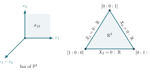
Boundary compatibility and Green functions
A function or form defined on the dense need not extend across these strata. The smooth tropical calculus imposes compatibility with projection to the lower-dimensional stratum: near the boundary, the form must come from that stratum in the directions that disappear. On , an ordinary smooth function in this sense is constant for all sufficiently large , locally near ; a positive-degree form vanishes there. A function such as instead has the affine growth expected of a Green potential for a boundary divisor.
This is why extended tropicalization contributes more than a compact picture. It records where a divisor lies and what growth a Green function must have. BGK25 develops the compatible delta-calculus, Green functions and star-products needed to compute local heights on a suitable tropical toric compactification. Its subdivision theorems and boundary conditions are additional results; the affine stable-intersection construction alone does not supply them.
There is a complementary global lesson. Over a complete, algebraically closed, nontrivially valued field, Payne’s theorem identifies the analytification of a quasiprojective variety with the inverse limit of its extended tropicalizations over all quasiprojective toric embeddings. One tropicalization forgets information; the compatible system recovers it. This topological reconstruction does not say that every current, metric or potential is represented on a single finite tropicalization.
References. [Pay09] (Theorem 4.2); [BGK25] (Sections 1.7–1.11 and 3). For a systematic further introduction, see [MS15].
Example 6.2.3. (Limits in the extended tropical plane). In the triangle coordinates above, the sequences , , and have respective limits The first sequence escapes through the interior of the cone generated by and reaches its zero-dimensional stratum. The second escapes along the ray and reaches the one-dimensional stratum . The third escapes along and reaches the one-dimensional stratum . A divergent sequence need not approach a toric fixed point.
6.3 Skeleta, slope formulas, and tropical degree
Skeleta of semistable pairs
For a strictly semistable pair , the skeleton is assembled from the standard simplices of local semistable equations, with unbounded directions contributed by the horizontal divisor . Its faces correspond to strata. The resulting integral-affine structure remembers the orders of vanishing of functions along model components and horizontal divisors.
In dimension one this is a metrized graph. In higher dimension, the normal direction along a codimension-one face carries data involving the neighbouring strata and intersection numbers. The higher-dimensional slope formula is therefore not obtained by summing arbitrary Euclidean normal derivatives. The model geometry specifies the correct weights and normalizations.
Slope formulas and principal divisors
If a rational function has divisor supported in the allowed boundary, its logarithmic absolute value restricts to an integral-affine function on each canonical cell of the skeleton. The slope formula expresses the balancing of its divisor data. On a curve it reduces to the familiar sum of outgoing slopes. In higher dimension it uses the incidence and intersection data of the semistable model.
This result is a bridge between algebraic principal divisors and tropical principal divisors. It tells us that the polyhedral data obtained from an analytic function obey the conservation law needed for integration. Conversely, an arbitrary PL function on a chosen skeleton need not be the logarithm of one analytic unit on a neighbourhood; lifting prescribed slopes is a separate problem.
The Sturmfels–Tevelev mechanism
For a generically finite map between suitable varieties in tori, the pushforward of the tropical cycle carries lattice-index weights. In a region where the map is combinatorially well behaved, the target weight is obtained by summing over source cells mapping onto the target cell, with the generic degree of the algebraic map accounted for in the cycle pushforward formula. This is the tropical version of counting sheets of a finite map, including ramification and multiplicity.
GRW develops related degree formulas for skeleta and tropicalizations. The lesson for CLD is direct: if a form is presented by a larger moment map and then projected, the calibrated integral must transform by precisely these degrees. The lesson for GK is equally direct: a tropical intersection product has to descend through the same refinement maps.
Existence and scope of faithful tropicalization
The faithful tropicalization theorem says that suitable rational functions can be chosen so that a specified skeleton is mapped injectively and unimodularly on its cells. It does not say that every tropicalization is faithful. Nor does it say that an arbitrary analytic datum factors through the retraction to that skeleton.
The distinction can already be seen on an annulus: the coordinate has slope and fails unimodularity when as an integer lattice index, while supplies the primitive parameter. Additional functions can separate cells that a first tropicalization identifies. In higher-dimensional proofs, constructing enough such functions is a geometric theorem involving models and rational functions.
The rational functions supplied for faithfulness may have divisors outside the original boundary divisor. Therefore the theorem should not be strengthened to a global factorization through the original skeleton without checking the actual functions and their domains.
Multiplicity one and the tropical skeleton
For a tropical fibre of multiplicity one, the unique Shilov boundary point gives a canonical candidate for a section of tropicalization. The continuity theorem in GRW applies on the multiplicity-one locus in its stated setting. The stronger uniqueness assertion for a continuous section includes an additional closure-of-interior hypothesis. These are different assertions.
The later paper Tropical Skeletons studies the collection of Shilov boundary points of tropical fibres and its topology and functorial behaviour. This is a more intrinsic construction relative to a tropicalization than simply choosing a semistable skeleton in advance. It helps explain when combinatorial points have canonical analytic lifts.
For the differential calculus, however, even a canonical section of one tropicalization does not eliminate all other charts. Equality of currents still requires every actual test. Chapter 24 explains why a topological inverse-limit theorem or a faithful section does not by itself transfer a Hodge theory.
References. [GRW16] (Theorems 6.12, 8.4, 9.5 and 10.6); [GRW17]; [Gub13].
Tropical contractions and SYZ fibrations.
Yamamoto’s 2026 theorem gives a further geometric use of tropicalization. For the Batyrev–Borisov degenerations over specified in [Yam26] (Section 3), with algebraically closed of characteristic zero, a good unimodular subdivision and irreducible generic fibre, tropicalization identifies the essential skeleton piecewise integrally affinely with the dual intersection complex. Composing with a tropical contraction gives an affinoid torus fibration off its discriminant, with the prescribed integral affine structure [Yam26] (Theorem 1.1). This is a structured degeneration theorem; it supplies no general descent theorem for CLD currents or cohomology.
6.4 Recovering an affine analytification from finite coordinate data
Payne’s theorem has a useful elementary core: every seminorm identity involves only finitely many functions. We prove a precise affine version using actual tropical images. This also identifies the point at which a topological reconstruction stops short of a differential or cohomological reconstruction.
Let be a finitely generated reduced -algebra and . Fix a finite set of algebra generators. Let be the directed set of finite subsets containing . The functions in give a closed embedding . Use absolute-value coordinates and set For , coordinate projection maps onto . With , the same construction takes values in . The value records a zero and is essential for embeddings into affine space.
NAG-900025 Proof review pending
Theorem 6.4.1. (Affine coordinate reconstruction). The natural map is a homeomorphism. Here the analytic space on the left is described by multiplicative seminorms on extending the absolute value of , and every is the actual image defined above.
Proof. A point in the inverse limit gives compatible numbers for every : choose a finite containing and read its coordinate. Directedness and compatibility show that the answer does not depend on the choice. For , choose one finite set containing . Its coordinate vector belongs to , so it is realized by an analytic point. Consequently Adding any to the finite set gives . Hence is a multiplicative seminorm extending , and determines a point of . Its image is the original compatible family. This proves surjectivity. If two analytic points have the same family, they have the same value on every , so they are the same seminorm. This proves injectivity.
Every coordinate of is an evaluation map, so is continuous. Conversely, the topology of is generated by all evaluations , and each of these is a coordinate projection from some . The inverse map is therefore continuous. No compactness assumption on is needed for this final step. ◻
The proof uses actual images, not an unproved identification with a combinatorial tropical variety. The theorem equating analytic images with algebraically defined tropicalizations is a separate input. Likewise, gluing affine descriptions into the toric-embedding formulation for a quasiprojective variety is the content of the global theorem cited in Section 6.1.5. Keeping these ingredients separate makes the reconstruction argument reusable.
NAG-900026 Proof review pending
Proposition 6.4.2. (Finite-coordinate neighbourhoods). Every ordinary neighbourhood of a point in contains a neighbourhood defined by finitely many conditions on values . On the open subset where all are nonzero, these conditions can be written using a finite tropicalization by analytic units.
Proof. The evaluation topology has a subbasis consisting of inverse images of open subsets of under single evaluations. Finite intersections form a basis, proving the first assertion. On the common nonvanishing locus, each regular is an analytic unit and the change of coordinate is a homeomorphism from to . This gives the second assertion. If some vanishes at the point, extended coordinates or a different local construction are required; deleting that coordinate would discard information. ◻
6.5 What a refinement must preserve
The preceding theorem recovers points and topology because their defining relations are finite. Differential forms involve an additional quotient: two presentations may agree after restriction to tangent spaces of the tropical support. Integration also involves weights, and current convergence involves a test topology. These three structures cannot be read from the underlying inverse-limit topology alone.
Example 6.5.1. (A homeomorphism that loses the lattice). The map , , is a homeomorphism and is integral affine, but its tangent-lattice map has index two. For a top superform , Thus topological injectivity does not give unimodularity, nor does it preserve calibrated integration with weight one. This is why faithful tropicalization includes an integral-affine requirement.
Example 6.5.2. (One tropical coordinate does not determine all tests). On the analytic torus with coordinate , the map forgets the values of for . On the open locus , the latter function is a unit and produces the additional smooth coordinate . Points with the same can have different . A test depending on this additional coordinate therefore need not be a pullback from the first tropical line. An identity checked only against functions of has not yet been checked against all original smooth tests.
To pass a calculation through chart refinements, one consequently needs: pullback preserving the quotient of forms; compatibility of and with that pullback; the weighted pushforward formula for integration; and continuity on the chosen spaces of compactly supported tests. Chapters 7–9 establish or explicitly import these ingredients in their stated categories. An inverse limit of spaces supplies none of them merely by being a homeomorphism.
The same distinction applies to cohomology. A direct limit of complexes requires actual transition maps of complexes. An identification with a complex on then requires exactness or a comparison argument, and a statement about cohomology requires a further passage through kernels and images. This is why a tropical Hodge theorem cannot be transferred to Berkovich cohomology solely by citing Payne’s topological theorem. It does not make such a transfer impossible; it specifies the additional mathematical work.
References. [Pay09] (Theorem 4.2); [GRW16] (Sections 9–10). The affine reconstruction above is proved directly for the explicitly defined system of actual images.
6.6 Tropical fibres and their Shilov points
Section 3.4 established the criterion for a singleton Shilov boundary. We now apply it to tropical fibres, using the formal-model comparison rather than identifying two different reductions. Now let be an integral closed subvariety of a split torus over a complete, algebraically closed, nontrivially valued field. For a tropical point with coordinates in the value group, the fibre is strictly affinoid. Its algebra is a quotient of a Laurent affinoid algebra. Distinguish its quotient Gauss norm from its spectral seminorm:
A quotient norm is submultiplicative and need not itself be an analytic point. The polyhedral formal model has the initial degeneration as special fibre; the canonical formal model has the canonical reduction as special fibre. The latter is reduced, and these two special fibres need not agree.
GRW Sections 10.2–10.5 supply a finite comparison of the two formal models and the associated special-fibre projection formula. Under equidimensionality, tropical multiplicity one forces a single component of the canonical reduction, hence a singleton Shilov boundary. The unique point is the spectral seminorm. Identifying it with the quotient norm requires the stronger reducedness condition on the initial degeneration. For arbitrary real , the valued-extension and boundary-descent results are additional inputs. This discussion separates the geometric theorem from the elementary norm argument above.
6.7 Adding coordinates without changing the lattice
NAG-900027 Proof review pending
Lemma 6.7.1. Let be a lattice. Suppose is injective with saturated image. For every integral map , the map has saturated image.
Proof. The cokernel of is finitely generated and torsion-free, hence free. Therefore admits an integral left inverse . Composing with projection onto the first factor gives an integral left inverse of :
The image of is thus a direct summand, in particular saturated. ◻
For tropicalizations, this lemma applies to each tangent lattice after taking a common integral-affine subdivision. It proves that adding coordinates preserves unimodularity wherever it was already established. The existence of a finite subdivision on a semistable skeleton is a separate assertion about the restrictions of rational functions.
Example 6.7.2. On an annular skeleton, the map is injective for every nonzero integer , but its lattice index is . The map is unimodular because projection to the second coordinate is an integral left inverse. More generally, is unimodular exactly when . Thus injectivity and preservation of the integral lattice are distinct requirements.
6.8 Finite separation on a compact skeleton
NAG-900028 Proof review pending
Proposition 6.8.1. Let be a compact polyhedral space, and let be a family of continuous real functions separating its points. Suppose a finite tuple drawn from is locally injective on and unimodular on a finite subdivision. Assume every further function is integral affine on a finite subdivision. Then a finite tuple extending gives a faithful embedding of into a real vector space.
Proof. Choose finitely many open sets covering such that is injective on each . Set
The set is an open neighborhood of the diagonal. Consequently is compact and contains no diagonal point. For every pair in , some function in separates and . The inequality persists on an open neighborhood of the pair. Compactness gives finitely many such functions which separate every pair in .
Together with these functions separate all points of : a pair in is separated by , and a pair outside by one of the added functions. Take a common finite subdivision. Lemma 6.7.1 preserves unimodularity on its cells. Finally, a continuous injection from a compact space into a Hausdorff real vector space is a homeomorphism onto its image. ◻
Remark 6.8.2. Local injectivity on is stronger than injectivity on each closed cell separately. Different cells meeting at a vertex may still be folded onto one another. Proposition 6.8.1 does not remove this hypothesis. Nor does its compactness argument apply directly to a noncompact skeleton with horizontal boundary.
In the GRW construction, semistable coordinates first supply integral-affine embeddings of individual canonical polyhedra. The global separation of different polyhedra uses additional rational functions and model geometry. Proposition 6.8.1 explains one possible finite assembly step when its stronger local hypothesis holds; it is not a replacement for the complete global theorem.
6.9 From faithful coordinates to differential calculus
Faithfulness concerns a specified subset of the analytic space. Its conclusions are injectivity and unimodularity on that subset. It does not say that every analytic function, smooth form, or current factors through a retraction onto the subset. A current is still tested on the full admitted test space, and a representative still requires compatibility under refinements.
The distinction matters already for a curve with good reduction: its smallest proper skeleton may be one point, while annular domains carry nonzero differential forms. Enlarging the system of charts recovers these directions. A finite faithful tropicalization of one skeleton therefore cannot by itself transfer a global Hodge or Green theory.
References. [GRW16] (Section 9 and Sections 10.1–10.6); [GRW17] (Sections 2 and 8).
6.10 Pure dimension away from the tropicalized boundary
A moment map on a -dimensional analytic space can have a lower-dimensional tropical image. Affinoidness and avoidance of the analytic boundary restore the expected dimension. The proof is useful beyond the dimension theorem: it turns a tropical projection into a finite morphism of affinoid spaces and then reads dimension at a Shilov boundary point.
NAG-900029 Proof review pending
Lemma 6.10.1. (A simultaneous integral projection). Let be a finite polyhedral complex of dimension at most , and let be contained in finitely many polyhedra of dimension at most . For , there is an integral linear map which is injective on every face of and satisfies . Assume that the stated finite polyhedral cover of consists of closed polyhedra, none containing .
Proof. For each face of , require to be injective on its tangent space . For each polyhedron in the chosen cover of , require injectivity on the linear span of . The first spaces have dimension at most , and the second have dimension at most . For each of these finitely many subspaces, injectivity is a nonempty open condition on the space of real matrices; its complement is given by vanishing of all relevant maximal minors and has empty interior. The intersection of the conditions is therefore nonempty and open. It contains a rational matrix. Clearing denominators gives an integral matrix without changing injectivity.
If had , choose a covering polyhedron containing . Then would lie in the kernel of on , a contradiction. ◻
In the analytic application, is compact and polyhedral, so a finite subdivision provides a closed polyhedral cover avoiding . The last condition in the lemma is material. Merely knowing that is not in a subset of a polyhedron would not imply that projection separates it from the whole covering polyhedron.
NAG-900030 Open proof obligation
Theorem 6.10.2. (Affinoid tropical purity). Let be complete and nontrivially valued, let be a strict affinoid space of pure dimension , and let be a moment map. Then has pure dimension at every point of
Open proof obligation (RC2). Prove the local germ and finite-projection step in the stated dimension, support and base-change scope; GRPL Theorem 6.4 and the proof of 6.6.
Remark 6.10.3. A constant moment map from a positive-dimensional proper space has a point as tropical image, although the source is boundaryless. This does not contradict the theorem, because the source is not affinoid. Conversely, a constant moment map from a positive-dimensional affinoid space sends its boundary to the same point, so the asserted open set is empty. Both hypotheses have visible roles.
This result concerns smooth tropicalization by analytic units. It does not prove purity of the image of a subvariety under the canonical tropicalization of a general abelian variety. That map comes from Raynaud uniformization and may forget an abelian part with good reduction. The distinction becomes important in Chapter 21, where canonical measures can live on cells of several dimensions.
References. [GRPL] (Sections 6.1–6.5 and Theorem 6.6). The proof above expands the finite-projection and Shilov-boundary argument; analytic dimension, properness, reduction and base-change results are explicit geometric inputs.
6.11 Matroids and the local models of tropical manifolds
Balancing is enough for Stokes, but not for all cohomological dualities. The matroidal local models used in tropical Poincaré duality satisfy a stronger incidence structure. This section constructs their fans from finite combinatorial data and proves balancing directly.
Definition 6.11.1. A matroid on a finite set is specified by a rank function satisfying , monotonicity, and submodularity Its closure is , with included. A flat is a set equal to its closure. A circuit is a minimal dependent set, where dependence means . We assume the matroid is loopless, meaning for every . Its rank is .
For vectors over a field, gives the basic example. The axioms do not require such a representation. Thus a matroidal tropical model need not arise from a linear subspace over the particular ground field under consideration.
NAG-900031 Proof review pending
Lemma 6.11.2. For , one has if and only if some circuit satisfies .
Proof. Choose a maximal independent subset of . Its cardinality is , and adding is dependent exactly when . In that case a minimal dependent subset of is a circuit and must contain , since is independent. Conversely, in a circuit , deleting any element leaves an independent set of rank . Thus , and closure is monotone, giving the assertion for . The facts about maximal independent sets and monotone closure follow from the rank axioms by adding one element at a time and applying submodularity. ◻
The circuit and flag descriptions
Let , where . Define the Bergman support by the minimum convention Adding a constant to all coordinates does not change this condition. For a nonempty proper flat , let be the class of its indicator vector. A flag of proper flats gives the cone
NAG-900032 Proof review pending
Proposition 6.11.3. The cones form a fan with support . If , this fan is pure of dimension . Each cone is unimodular in the lattice of its linear span.
Proof. A weight satisfies the circuit condition exactly when each nonempty proper upper level set is a flat. If such a level set is not flat, choose in its closure. Lemma 6.11.2 gives a circuit contained in , with its unique minimum. Conversely, a unique minimum in a circuit is separated from the other circuit weights by a level , making lie in the closure of but not in .
The distinct upper level sets form a nested flag. Subtracting the minimum weight expresses uniquely as a positive linear combination of their indicator vectors. Allowing some coefficients to vanish gives the faces of the cones. Thus intersections of cones are their common flag faces, proving the fan assertion. Strict inclusions of flats increase rank. Every flag can be filled to one containing a flat of each rank , by adjoining an element outside the current flat and taking closure. Hence maximal cones have generators.
To check the lattice, put , , and choose an element for . For , the integral coordinate difference descends to and takes the value on . These differences give an integral left inverse to the generator map . Its image is saturated, proving both linear independence and unimodularity. ◻
NAG-900033 Proof review pending
Theorem 6.11.4. (Weight-one balancing). Assign weight one to each maximal cone of the flag fan. The resulting weighted fan is balanced.
Proof. A codimension-one flag omits exactly one rank between two successive retained flats , with ; allow and . The maximal cones containing it correspond to intermediate flats of rank . In the rank-two minor , the sets are its rank-one flats. They partition : each element has a unique rank-one closure, and two such closures either agree or are disjoint. If there are of them, their indicator vectors satisfy Modulo the span of the codimension-one cone, the right side vanishes; when , its vector already vanishes in . By the preceding unimodularity argument, the image of each is the primitive outgoing generator for its adjacent cone. Thus the displayed identity is exactly the balancing equation with all weights one. Rank one has no balancing faces to check. ◻
The proof uses only the rank-two intervals in the lattice of flats. This explains why matroidal fans have particularly controlled local stars. It also separates two uses of the word smooth: a unimodular cone is a lattice property, whereas being a tropical manifold requires every local model to have the specified matroidal form. A fan all of whose individual cones are unimodular need not have that local form.
References. [AK]; the use of these local models in tropical Poincaré duality is [JSS] (Definition 4.15 and Theorem 4.33).
6.12 Accessible skeleta and the limits of functoriality
A semistable skeleton is constructed from a model and comes with its associated retraction. The tropical skeleton of a fixed torus embedding is defined through Shilov boundary points of tropical fibres. Neither description by itself supplies a class stable under all the operations needed in analytic geometry. Ducros–Thuillier introduce accessible skeleta to address this functorial problem. We retain the coefficient data and the -strict category of their paper. Locally in the -topology, an accessible skeleton is covered by compact pieces that are images of elementary classical skeleta under analytic morphisms into compact analytic domains. The image is not required to consist only of points with maximal possible Abhyankar rank in the target. This is one reason the accessible category is larger than the classical category.
NAG-900034 Open proof obligation
Theorem 6.12.1. (Ducros–Thuillier, fixed version). In the category of [DT26], accessible skeleta form the smallest admissible class containing the standard torus skeleta. This class contains classical skeleta, is stable under finite intersections and the specified piecewise linear subspaces, and has the following functorial properties.
If and is accessible, with topologically proper, then is accessible.
If is accessible and every fibre over is empty or zero-dimensional, then is accessible.
The function is locally constant on an accessible skeleton. Its locus where is open and closed and is classical.
Open proof obligation (RC2). Prove the accessible-skeleton geometric image assertion; this block explicitly offers DT26 and APW26 as imported proof.
An accessible skeleton is not, by its definition, a deformation retract of the ambient space. Nor does the image theorem assign the tropical multiplicities needed to push differential forms. To use it in an integration formula one still needs weights, lattice normalizations and compatibility with calibration. To use it in a Green-form construction one additionally needs descent in the chosen sheaf of actual forms. These are separate inputs. There is a further distinction from faithfulness. Faithful tropicalization concerns the behaviour of a chosen map on a chosen skeleton. In the strong faithfulness used in [APW26], injectivity on the relevant dual complex is supplemented by weight one on its top-dimensional tropical faces. The additional weight condition allows multiplicity formulas to control other branches above generic tropical points. A homeomorphism on the chosen skeleton alone supplies no such control.
References. [DT26] (Theorems 9.1.12 and 9.2.3); [APW26] (Section 12.4).