5.1 Tropicalization of subvarieties of a torus
Throughout these foundations, is a complete non-Archimedean field with a nontrivial absolute value. We write Algebraic closure will be stated when needed; it is a standing hypothesis of GK17, not a consequence of completeness. The real polyhedral constructions below do not themselves involve a field. We retain the series normalization , without a factor and without squaring a norm.
Cancellation and repeated minima
Suppose that , with each , in a non-Archimedean valued field. The smallest of the numbers must occur at least twice. Indeed, if had strictly smaller valuation than all the others, then a contradiction. This observation also applies to evaluation at a Berkovich point: all the evaluated terms lie in its completed residue field .
Let . For a nonzero Laurent polynomial where only finitely many are nonzero, define This is a continuous, concave, piecewise affine function on . Concavity follows because it is the minimum of affine functions. Its tropical hypersurface is the set where that minimum is attained for at least two distinct exponents. The word hypersurface denotes this set with suitable multiplicities, not the graph of .
At an analytic point , put If , the preceding argument proves that belongs to the tropical hypersurface of . For arbitrary , the ultrametric inequality gives only Equality can fail because terms of equal size can cancel. We will obtain equality at the particular Gauss points of Section 6.1. It must not be used at every analytic point.
The tropical line
Example 5.1.1. (The MIN tropical line). For , all three coefficients have valuation zero, so Two terms can be minimal in exactly the following three ways: Their union will be denoted by . Each ray has weight one; the meaning of this weight is explained in the next section.
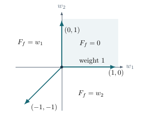
This calculation is worth doing before memorizing a familiar tropical-line diagram. With the convention , the rays point right, up, and southwest. On the first quadrant the constant term is smallest. On the left-hand region the -term is smallest, and on the lower region the -term is smallest.
Definition 5.1.2. (Tropicalization of a closed subscheme). For a closed subscheme , its set-theoretic tropicalization is The scheme structure will enter through the weights, even though this underlying set does not detect nilpotents.
NAG-900008 Proof review pending
Theorem 5.1.3. (Polyhedrality and the hypersurface theorem). For a closed subscheme , the set is a finite union of integral -affine polyhedra. If is pure of dimension , this union can be made into a pure -dimensional polyhedral complex. If for a nonzero Laurent polynomial, then is exactly the locus of repeated minima of .
Here the definition uses all Berkovich points. It requires no assertion that a prescribed real valuation vector is realized by a -rational point. Over an algebraically closed nontrivially valued extension , one can instead take the closure of the coordinatewise valuations of . The converse implication in the hypersurface assertion is a theorem about lifting tropical data, not a consequence of the ultrametric inequality alone.
References. [Gub13] (Theorem 3.3, Proposition 3.8, Theorem 5.6 and Example 5.8). The guide treats arbitrary valued ground fields and performs analytification over their completions. The elementary argument above proves the necessary cancellation condition.
For an ideal with several generators, intersecting the tropical hypersurfaces of those generators gives a tropical prevariety. It may be larger than . The fundamental theorem uses the whole ideal, or a specially chosen finite tropical basis. A generating set for the ordinary ideal need not be a tropical basis.
Example 5.1.4. (Tropical prevarieties and translation). Assume . The polynomials and have the same tropical polynomial . Their tropical hypersurfaces therefore agree. Nevertheless, , so is the unit ideal and is empty.
More generally, for , the tropical hypersurface of is a translate of the standard tropical line. Subtracting from the three term valuations gives Its vertex is . Translation changes the vertex but preserves the primitive directions and the weights, which are one.
5.2 Lattices, polyhedra, multiplicities, and balancing
Character lattices and integral affine structures
The expression is intrinsic to the torus even though its coordinate notation is not. Let Thus is the character lattice and its dual, the cocharacter lattice. Write for the character associated to . Tropicalization is characterized without coordinates by A torus homomorphism induces an integral linear map on cocharacter lattices and hence a real linear map on tropicalizations. Translation by a torus point adds a constant valuation vector. These are the origins of the integral affine changes of coordinates used throughout GK17.
Definition 5.2.1. (Integral affine data). An integral -affine function on is a function , with and . An integral -affine polyhedron is an intersection of finitely many half-spaces Allowing gives integral -affine polyhedra. A polytope is a bounded polyhedron. A face is the polyhedron itself or its intersection with a supporting hyperplane. The relative interior means interior in the smallest affine space containing the polyhedron.
The adjective integral controls slopes, not the coordinates of every vertex. For example, is an integral -affine inequality when ; its endpoint need not lie in . In general, vertices may lie in the divisible hull of . This distinction is relevant to strict analytic domains and to model metrics over a fixed ground field.
A finite polyhedral complex contains every face of each of its cells, and the intersection of two cells is empty or a face of both. Its support is their union. It is pure -dimensional if every maximal cell has dimension . A subdivision cuts cells into smaller cells without changing the support. The underlying tropical cycle will not depend on such cuts.
For a cell , let be the vector space parallel to its affine span and put For a facet of , the quotient is a free rank-one lattice. Its generator pointing from into is a primitive normal class. Choose a lift . Another lift differs by an element of .
Primitive refers to the lattice: a vector cannot be a positive integer multiple of another lattice vector on the same ray. It does not mean Euclidean length one. For instance, is primitive, and the natural integral coordinate on its line is ; its Euclidean length plays no role in a tropical multiplicity.
References. [GK17] (Appendix A.1–A.6 and Definition 1.1); [Gub13] (Appendix A.1–A.4).
Tropical multiplicities
The reason for attaching weights is already visible in one variable. The scheme has length , while its tropicalization is the single point . That point must carry weight to retain the algebraic degree. This remains true if the scheme is nonreduced, for example when the characteristic divides .
In higher dimensions, the relevant algebra is an initial degeneration. Here is a construction that does not assume a chosen section of the valuation. For , pass to a valued extension and choose with . Translate by , take its schematic closure in the split torus over , and take the special fibre. The result is denoted . Different choices give equivalent schemes after residue-field extension and torus translation.
For a Laurent polynomial, this operation retains the terms attaining the minimum in (5.1.1), after rescaling them to have valuation zero, and reduces their coefficients. For an ideal, one takes the initial forms of all its elements. The fundamental theorem says In the Laurent coordinate ring, a monomial is a unit. Thus an initial ideal containing a monomial defines the empty scheme.
At a regular point of , lying in the relative interior of a maximal cell, its tropical multiplicity is the sum of the multiplicities of the geometric irreducible components of . An irreducible-component multiplicity means the length of the local ring at its generic point. Passing to an algebraically closed residue-field extension ensures that geometric components are counted. This integer is locally constant on the regular locus and therefore gives a weight to each maximal cell.
Example 5.2.2. (A binomial weight). Let , with primitive and , and consider Its tropicalization is the hyperplane , with weight . Extend to a basis of ; in the resulting coordinates the equation is . Its initial degeneration is a product of a zero-dimensional scheme of length with a torus of dimension . Thus the weight is a scheme-theoretic multiplicity, including repeated roots, rather than a count of distinct points.
References. [Gub13] (Definitions 5.1 and 13.4, Remark 5.7, Theorems 5.6 and 13.8).
Computing an initial ideal: why all relations matter
The phrase “keep the lowest-weight terms” first defines for a single polynomial. For , the geometric object is instead determined by with the coefficient normalization made over a suitable valued extension as above. A generating set of need not be a tropical basis or a Gröbner basis at .
Here is a calculation at . Assume the residue characteristic is not , choose , and work in . Let The initial forms of these two displayed generators both equal . They define a line in the residue torus. But Thus , and its initial degeneration is the single residue-torus point . Taking initials of only the two original generators loses a relation and even gives the wrong dimension.
The construction by translation and closure is useful precisely because it is intrinsic to the ideal. A coefficientwise computation is reliable when one knows a suitable basis, or proves directly that the proposed initial generators generate the entire initial ideal.
Generic weights and cell multiplicities
To attach the weight to a maximal cell , choose in its relative interior in a subdivision on which the initial-degeneration type is controlled. This is a regular point of the tropical support: locally that support is a piece of an affine space of the expected dimension. Moving inside that regular region does not change its multiplicity.
For balancing at a codimension-one face , there are several neighbouring maximal cells. Each carries the weight computed on its own relative interior. A point of is useful for studying the entire local star, but it is not substituted for all these interior points in the definition of their weights. The multiplicity function need not be described as one locally constant function across every singular face of the support.
The algebraic origin of balancing
For the tropical line, three primitive vectors sum to zero. For a hypersurface, the dual Newton subdivision often makes the balancing identity an elementary polygon calculation. Neither argument proves the theorem for an arbitrary higher-codimension ideal.
The general proof relates the star near a point to the tropicalization of an initial degeneration. After this reduction, the balancing relation is an intersection-theoretic degree identity. Roughly, a character defines a principal divisor on an appropriate toric compactification; its intersection degree with the relevant proper cycle is zero. The contributions along the toric boundary are the multiplicities times the primitive normal components. Their sum is therefore zero. Passing back through the initial degeneration recovers the balancing equation for the original tropicalization.
This is a proof mechanism, not a replacement for the compactification and multiplicity arguments in [Gub13] (§13, Theorem 13.11). It explains the content of the theorem: the algebraic multiplicities satisfy a compatibility that arbitrary weights on the same support would not satisfy. Once balancing is known, Stokes translates it into closedness of the integration current.
The balancing condition
Definition 5.2.3. (A balanced tropical cycle). Give each maximal cell of a pure -dimensional integral -affine complex an integer weight . The complex is balanced if, for every -dimensional face , Equivalently, the sum is zero in . With integer weights it lies in . A tropical cycle identifies balanced weighted complexes that agree after subdivision; cells of zero weight do not contribute to its support.
For a curve, is a vertex and . Balancing says that the weighted sum of primitive outgoing direction vectors is zero. The tropical line satisfies An arbitrary graph drawn with straight edges need not satisfy this equation. Conversely, a balanced weighted graph is a valid abstract tropical cycle even when no algebraic realization has been specified.
NAG-900009 Open proof obligation
Theorem 5.2.4. (Balancing of algebraic tropicalizations). If is a pure-dimensional closed subscheme of a split torus, its tropical multiplicities make a balanced tropical cycle of dimension . The resulting cycle is independent of the chosen polyhedral subdivision.
Open proof obligation (RC2). The sole supplied proof source for the stated algebraic tropical balancing/subdivision claim is GubGuide Theorem 13.11 and Remark 13.12.
Later, integration over a constant-weight cycle will define a current . Balancing is precisely the cancellation of facet terms that makes this current - and -closed. This explains why the combinatorial condition belongs in a differential theory. GK17 also allows smoothly varying real weights, with a pointwise balancing equation. In that setting derivatives of the weights remain inside the cells: balancing alone does not imply that is closed [GK17] (Proposition 2.16). We will retain constant weights until that distinction has been explained.
Example 5.2.5. (Primitive directions and lattice index). For the rays with primitive directions , balancing is The smallest positive integral weight vector is . Replacing the primitive directions by Euclidean unit vectors changes their normalization and hence the coefficients in the balancing equation.
The cone generated by and is simplicial, since the two vectors are linearly independent. Their determinant is two, so the lattice they generate has index two in . Simpliciality does not imply unimodularity.
Example 5.2.6. (A binomial of multiplicity two). Let . The tropical support of is The exponent difference is , with primitive. The weight is therefore two. Equivalently, use the primitive character ; the transverse equation is and has length two. In residue characteristic two the initial transverse scheme can be nonreduced, but its length remains two. Counting distinct geometric roots would lose this multiplicity.
5.3 Initial degenerations and multiplicity calculations
Initial degenerations over valued extensions
Let , let , and let have ideal . Fix . The valuation of a Laurent term at weight is If is realized by a torus point over a suitable valued extension, substitute . For each relation, divide by an element whose valuation is the minimum of its term valuations, then reduce. The terms attaining the minimum survive; the others vanish in the residue field. The ideal generated by all these reduced relations defines the initial degeneration.
This description explains why one sometimes extends the field before writing an initial ideal with ordinary residue coefficients. A weight in need not lie in the original value group. Graded reduction or the corresponding tilted algebra packages the same information without pretending that every real weight is realized by a point over the original field. The eventual tropical multiplicity must be invariant under the permitted extensions and choices.
A nonempty variety whose chosen equations give a larger prevariety
Consider the ideal in three Laurent variables The variety is nonempty: it is given by and , inside the torus. At the weight , the two displayed generators both have their minimum attained by the terms and . Thus this weight belongs to the intersection of their two tropical hypersurfaces.
But subtracting the equations gives . At the same weight, its constant term has value and its term has value . Its initial form is the nonzero constant . Therefore the full initial ideal is the unit ideal, and the weight is not in .
This example isolates the issue without an empty algebraic variety: solving the minimum-tie condition for a chosen generating set does not necessarily impose the minimum-tie condition for every algebraic relation. The intersection of the chosen tropical hypersurfaces is a tropical prevariety; obtaining the actual tropical variety requires a tropical basis or another method controlling the full initial ideal.
A multiplicity calculation that keeps nilpotents
For the one-variable equation , the tropical support is the point . After a suitable translation and residue extension, the initial equation is with . Its zero-dimensional length is . If the residual characteristic divides , the polynomial can be inseparable and some geometric roots can coincide. The sum of scheme-theoretic multiplicities is still .
Thus a tropical multiplicity is not generally the number of distinct geometric roots of an initial equation. It counts lengths at generic components. This is why taking a reduced initial degeneration before measuring multiplicity can give the wrong answer.
In higher dimension, at a regular point of a maximal tropical cell, the initial degeneration has a torus symmetry parallel to the cell. Quotienting by that tangent torus leaves a zero-dimensional transverse scheme. Its length is the conceptual source of the cell weight. The algebraic construction makes this description invariant under the choices needed to realize the weight.
For the hypersurface defined scheme-theoretically by , the support of the tropicalization is unchanged but its generic multiplicity is two. This is a useful distinction between a reduced support and a cycle. If one first replaces the subscheme by its reduction, the cycle changes. The multiplicity is not inferred from the picture of the three rays.
Why the weight is constant only in the appropriate region
The initial degeneration can change when crosses a Gröbner wall. On a sufficiently fine polyhedral subdivision, the relevant initial data are constant in the required sense on relative interiors. The tropical multiplicity is locally constant on the regular locus of a maximal cell. At a lower-dimensional face, several maximal cells meet and there is no single weight to obtain by pretending that the face is a generic point of one chosen cell.
When defining the weight attached to , choose in its relative interior away from the lower-dimensional exceptional locus. When proving balancing at a face , choose a point in the relative interior of and examine the local star, with the weights already assigned to adjacent maximal cells. These are two different choices of point serving two different purposes.
A proof mechanism for balancing
Near a codimension-one face, quotient the local star by the tangent space of that face. The transverse geometry is one-dimensional. In the corresponding initial-degeneration picture, characters of the quotient torus give rational functions on a compactification of the relevant curves. A principal divisor has degree zero. Its orders at the boundary points are the pairings of the character with the primitive outgoing directions, weighted by the transverse multiplicities. Hence, for every quotient character , Characters separate vectors in the quotient real vector space, so the weighted normal sum vanishes. This explains the algebraic source of balancing. Making the argument general requires the initial-degeneration, compactification, and multiplicity theorems; the vector identity is its conclusion, not an extra combinatorial assumption about an algebraic tropicalization.
Example. (Valuation of a coefficient). For , the tropical polynomial of is . Its repeated-minimum locus is the standard tropical line translated by . Its vertex is , and the outgoing primitive directions remain , all with weight one. The coefficient valuation affects position, not the tangent lattices.
References. [Gub13] (Sections 5–6, 10–13); [MS15].
5.4 Corners and stable intersections
Corner divisors
On a weighted tropical curve, a continuous piecewise affine function has a divisor at its vertices: Here is differentiation in the primitive lattice coordinate pointing away from , and subdivision inserts vertices at all breakpoints. This is the outgoing-slope convention used throughout the series. On the line, The coefficient is the right derivative minus the left derivative. These are the previously studied atomic-curvature calculations in a tropical divisor notation.
In higher dimension, a normal vector is defined only modulo a tangent vector. A formula must compensate for this ambiguity.
Definition 5.4.1. (The corner divisor). Let be a constant-weight tropical cycle and let be continuous and affine on every cell of a subdivision. Denote the linear part of its restriction to by . The weight of on a facet is Integral slopes give integral divisor weights when the weights of are integral. Real slopes are also allowed, with real divisor weights.
Balancing puts the vector in the second term in , where is defined. Replacing a lift by , with , changes the first term by and the second by . These agree because is continuous along . Hence the formula is independent of the lifts. If is the restriction of one ambient affine function, the two terms cancel completely.
The resulting divisor is again balanced and is independent of subdivision. This is a substantive compatibility theorem; it makes it possible to iterate corner operations. The same construction in GK17 applies to piecewise smooth functions and smooth weights, using derivatives at each point of the face.
References. [GK17] (Definition 1.10, Remark 1.11 and Propositions 1.12–1.14); Section 10.3.
There is a useful analytic dictionary. For constant-weight , when is piecewise affine and the currents are taken on . For a piecewise smooth function there is also the facewise Hessian: Thus differentiating each affine piece and obtaining zero does not compute the derivative of the whole current. The missing terms live on the interfaces.
References. [GK17] (Corollaries 3.19–3.20).
Example 5.4.2. (The sign of a tropical polynomial). The tropical polynomial in (5.1.1) is concave. Consequently the effective tropical hypersurface is the corner divisor of , not of . Near a general facet where two exponents differ by , with primitive, the slope jump of in a transverse integral coordinate is . This recovers the binomial multiplicity.
In particular, for the tropical line, This statement is on the real tropical chart. It does not replace the analytic function by at points where cancellation occurs.
Example 5.4.3. (The correction term in the corner formula). Subdivide along , with both weights one, and use normal lifts and . For , formula (5.4.2) gives For , it gives Thus the affine function has no corner, whereas the second function has divisor . The correction along the common tangent space is exactly what removes the dependence on the chosen lifts.
Example. (Slopes on the tropical line). Give the three rays outgoing slopes , using their primitive parameters. The coefficient of the corner at the central vertex is . For the restriction of an ambient affine function , these slopes are , so the sum is zero. For a general piecewise affine function they need not sum to zero. In particular, slopes give negative curvature at the vertex although the function is affine, hence convex, on every ray.
This calculation is the simplest reason the continuous facewise-convexity criterion in CLD12 requires correction. A condition on each maximal cell does not control the terms on their interfaces. Appendix A gives the exact source locator and the corrected interpretation.
Stable intersection of tropical cycles
Two coincident lines have a one-dimensional set-theoretic intersection, whereas the intersection of two codimension-one cycles in a plane should have dimension zero. Tropical geometry resolves this discrepancy by a displacement procedure.
For cycles , translate by , with generic and small, intersect transverse faces, and take the limiting cycle as . When cells meet transversely in complementary dimensions, their contribution has multiplicity The index counts how far the two integral tangent lattices are from generating the ambient lattice. It is finite under the stated transversality condition. For two primitive lines in , it is the absolute determinant of their direction vectors.
NAG-900010 Proof review pending
Theorem 5.4.5. (Stable intersection). For constant-weight integral -affine tropical cycles in , the displacement construction defines a cycle , independent of the sufficiently small generic displacement and of subdivision. It is bilinear, associative and commutative, its codimension is the sum of the codimensions, and its support is contained in . The construction extends to real weights and to the smooth weights used by GK17.
Independence of displacement uses balancing. It is not a general fact about arbitrary weighted polyhedral sets. The combinatorial intersection is defined before any attempt to multiply singular currents.
References. [GK17] (Sections 1.3–1.4, especially formula (1.4.1)).
Example 5.4.6. (A transverse intersection of multiplicity two). In , give each of the lines weight one. Their primitive tangent vectors are and . They generate the sublattice of vectors with even first coordinate, of index two. Hence The corresponding algebraic example is Its coordinate algebra is , of length two. In characteristic two the two roots merge into a nonreduced point; the intersection length and tropical index remain two. Both individual tropical lines have weight one because their defining exponent vectors and are primitive.
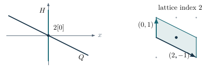
The same index will appear in products of curvature currents. With and , the corner cycles are and . Their product in the delta-calculus is therefore . This formula is justified by that calculus; it is not a definition of the product of two arbitrary distributions.
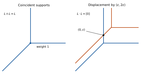
Example 5.4.7. (Two different self-intersections). A straight line translated in a nonparallel direction becomes disjoint from itself, so its stable self-intersection is zero. The tropical line behaves differently. Translate its vertex by . There is one transverse intersection, at , between the original vertical ray and the translated southwest ray. Their primitive directions have determinant of absolute value one. Letting gives Although both set-theoretic self-intersections contain the entire original curve, the stable answers differ.
Example 5.4.8. (Determinants and intersection multiplicities). Let and be primitive integral covectors with . The weight-one lines and have primitive tangent vectors and . Their stable intersection is the origin with weight The torus homomorphism has the same degree. Indeed, its character-lattice map has cokernel of order , so its finite kernel has that scheme-theoretic length. The formula remains valid in inseparable characteristic, where the kernel need not be reduced.
Example. (A nontrivial lattice index). Let two weighted rational lines in have primitive directions and , with weights and . A generic small translate meets transversely, and the stable intersection multiplicity is The factor two is an index of integral tangent lattices. It is not the angle between the lines. If the two lines coincide, their set-theoretic intersection is one-dimensional, whereas the stable intersection is defined by a displacement construction and the expected codimension. This is why ordinary intersection of supports cannot be substituted for tropical intersection of cycles.
5.5 Weighted Gauss points and the role of cancellation
The tropical image contains real vectors which need not be valuations of -rational points. Weighted Gauss seminorms explain this already for a torus, without changing the ground field.
NAG-900011 Proof review pending
Proposition 5.5.1. Let be a complete non-Archimedean field, , and . The rule is a multiplicative norm extending that of . It determines a point of the analytified torus, and . The map is continuous.
Proof. Choose a basis of and put . The Laurent-polynomial case of Proposition 1.2.2 gives multiplicativity with these radii.
The norm is nonzero on every nonzero polynomial and has the specified values on characters. These facts give the analytic point and its tropicalization. Continuity follows from the topology of analytification: evaluation of each Laurent polynomial along is the maximum of finitely many continuous functions. ◻
At these points one has . At a general analytic point with the same tropicalization only the inequality holds. Thus is a section on the torus, but it is not a section on every subvariety: if vanishes on a subvariety, the Gauss norm of a nonzero remains nonzero. A point of the subvariety over must carry cancellation information absent from the torus Gauss point.
5.6 Primitive lattices and the index in a pushforward
NAG-900012 Proof review pending
Lemma 5.6.1. If is a rational linear subspace, then is saturated in . If are rational subspaces with dimension difference one, is free of rank one.
Proof. If for a nonzero integer and , then , so . Thus the quotient has no torsion. The same argument inside proves that is torsion free. Its rank is the dimension difference, since both subspaces are rational. A finitely generated torsion-free abelian group of rank one is infinite cyclic. ◻
NAG-900013 Proof review pending
Proposition 5.6.2. Let be integral linear and injective on the span of a -dimensional rational polyhedron . Let and For a compactly supported -superform on the relative interior of one has
Proof. Choose bases of the two tangent lattices. The resulting square integral matrix has nonzero determinant and . Pullback acts on both exterior factors, so the top-form coefficient is multiplied by . The ordinary change of variables in the scalar integral contributes . Their product is . The sign convention for top superforms is the same on both sides and does not introduce an orientation sign. ◻
For finitely many maximal cells mapping onto one image cell, summing this formula produces the weight . This explains the lattice factor in tropical pushforward and integration. Identifying that weighted pushforward with the tropicalization of an algebraic image, divided by the generic algebraic degree when appropriate, requires the Sturmfels–Tevelev multiplicity theorem. The change-of-variables calculation does not prove that algebraic theorem.
Example 5.6.3. For a nonzero integer and on the tropical line, . Integration gives . The same factor is the degree of the torus isogeny . If the characteristic of the fibre field divides , distinct geometric points need not count that degree; scheme lengths do. For an initial fibre this is the residue characteristic. An isogeny over a characteristic-zero ground field remains separable even when its degree is divisible by the residue characteristic.
5.7 Monomial maps and scheme-theoretic degree
The lattice indices in tropical intersection are algebraic degrees. The following calculation proves this for a general isogeny of split tori, including inseparable characteristic. It also distinguishes the multiplicity of an initial degeneration from the number of geometric points in a generic fibre.
Let and be free abelian groups of rank , and let be injective with finite cokernel. Over any field , the inclusion of group algebras gives a morphism
NAG-900014 Proof review pending
Proposition 5.7.1. The map is finite faithfully flat of degree . Every fibre algebra has vector-space dimension over the residue field of the target point.
Proof. Choose one representative from each coset in . Every monomial has a unique expression , so as a module over . Independence follows because distinct monomials form a -basis of the group algebra. Hence this algebra is finite free of positive rank , and thus faithfully flat. Tensoring with the residue field of a point of produces a -dimensional algebra over that field. It is finite, hence zero-dimensional, and its dimension is its scheme length with residue degrees counted. ◻
NAG-900015 Proof review pending
Proposition 5.7.2. (Smith normal form and inseparability). After integral changes of bases, is the map and . Over an algebraically closed field of characteristic , write with . Each geometric fibre has distinct points, each of length . In characteristic zero every geometric fibre is reduced with points.
Proof. Smith normal form is the integer row-and-column reduction of a full-rank integral matrix to the displayed diagonal matrix. The basis changes are torus automorphisms, so they preserve the fibre schemes and degree. In one coordinate, after choosing a th root of the nonzero target coordinate, The polynomial has distinct nonzero roots, since its derivative does not vanish at any root. The local quotient at each root is isomorphic to and has length . Tensoring these one-coordinate algebras proves the count and the length in coordinates. The same derivative argument with applies in characteristic zero. ◻
This statement uses the characteristic of the field over which the fibre is formed. If has characteristic zero and residue characteristic , the isogeny has reduced geometric fibres over , while its reduction can have a nonreduced fibre of length . The total degree is in both calculations; the source of multiplicity differs. Tropical multiplicity uses the appropriate initial degeneration over a residue field.
5.8 Binomial complete intersections and tropical weights
Return to a complete non-Archimedean field . Let be linearly independent elements of , let , and set
NAG-900016 Proof review pending
Theorem 5.8.1. The scheme is finite of length . Its tropicalization is one point , uniquely determined by This point has tropical multiplicity . The conclusion includes nonreduced schemes and weights outside the original value group.
Proof. The equations define the fibre of the isogeny associated with the sublattice generated by the , over the point . Proposition 5.7.1 proves the length and nonemptiness. Every analytic point of satisfies the displayed valuation equations. They have a unique real solution because the form a real basis. A finite nonzero -algebra has a maximal ideal with finite residue extension of ; the extended absolute value gives an analytic point. Thus the tropicalization is exactly .
Choose a valued extension containing a solution of the binomial system. Translation changes the equations to . The closure of this kernel in the torus over the valuation ring is finite free of rank : the same coset-basis proof works over a ring, and imposing the target coordinates equal to one preserves that free basis. Its generic fibre is the translated , and it has no valuation-ring torsion. Hence it is the schematic closure. Its special fibre has dimension as a vector space over the residue field. After algebraic closure of that residue field, the sum of local lengths is still . This is exactly the tropical multiplicity in dimension zero. ◻
NAG-900017 Proof review pending
Corollary 5.8.2. (Transverse hypersurfaces). The stable product of the tropical binomial hypersurfaces is , equal to the tropical cycle of .
Proof. Write with primitive. The th hypersurface has weight . The primitive normal covectors are real-linearly independent. The transverse lattice-index rule gives multiplicity for the weight-one hyperplanes; multiplying their weights gives . The support is their unique intersection point . This uses the transverse part of the tropical intersection construction, not a general lifting theorem for intersections. ◻
Example 5.8.3. Consider in a three-dimensional torus the equations The exponent matrix has determinant , so the intersection has length . Its tropical point satisfies The first hypersurface has weight two. The other two exponent vectors are primitive and give weight-one hypersurfaces. Their three primitive normal vectors have determinant ; multiplying by the weight two recovers . Thus neither the individual weights nor the primitive intersection index alone gives the answer. The computation remains valid in characteristics two, three and five.
For non-binomial equations, a transverse intersection of tropical supports need not by itself identify an algebraic scheme intersection without the relevant lifting and proper-intersection hypotheses. The binomial proof succeeds because one finite free algebra controls both the generic fibre and the initial fibre. In the general theory, flatness, initial degenerations and multiplicity comparison replace that explicit algebra. This is the point at which the geometric results used by Gubler and collaborators enter the calculus.
References. [Gub13] (Sections 5 and 13); [GK17] (Section 1). The finite-free and initial-fibre calculations are proved here; the general tropical multiplicity and intersection conventions are those of the cited sources.
5.9 Real weights and valued extensions
A tropical point is a real vector; it is not required to be the valuation vector of a point over the original ground field. There is a direct construction of a complete valued extension realizing any prescribed vector. It explains why the definition by initial degenerations remains meaningful for arbitrary real weights.
NAG-900018 Proof review pending
Proposition 5.9.1. For every , there is a complete valued extension and elements with . The absolute value on restricts to the given one on .
Proof. On the Laurent polynomial ring take the weighted Gauss norm It is multiplicative. One proof uses the associated graded ring: the initial homogeneous part of a nonzero polynomial is nonzero, and the graded Laurent polynomial ring over the graded residue field is a domain, so initial parts of a product cannot multiply to zero. Equivalently, refine the real weight order by a monomial order to select a leading exponent; the leading coefficients multiply without cancellation. Extend the norm to the fraction field by , then complete. The images of have the prescribed norms, while constants keep their original norms. ◻
This is a valued extension construction, not a finite-extension assertion. A finite extension cannot introduce an arbitrary real value over a discretely valued field: its value group remains a finite-index enlargement. Thus strictification by a general analytic extension and descent through a finite field extension are different operations.
5.10 The closure algebra and all initial relations
Fix as above and put , and . Translate the given subscheme by , so its ideal becomes . The closure algebra in the torus over is
NAG-900019 Proof review pending
Proposition 5.10.1. The algebra is torsion-free over and hence flat over this valuation ring. Its special-fibre ideal is generated by the reductions of all normalized polynomials in : divide each nonzero polynomial by one of its coefficients of maximal absolute value and then reduce.
Proof. The map is injective by the definition of . Its target has no -torsion, because every nonzero element of is invertible in . Thus is torsion-free. We use the standard valuation-ring criterion that every torsion-free module is flat.
A normalized polynomial has coefficients in , with at least one unit coefficient, so it belongs to and reduces to a nonzero initial polynomial. Conversely, take . If all its coefficients belong to , its reduction is zero. Otherwise a coefficient of maximal absolute value is a unit of ; dividing by that coefficient changes its reduction by a nonzero scalar in and gives one of the stated normalized relations. These two observations identify the ideals in . ◻
The proof shows why dividing by a small scalar is necessary even if it is not a unit in . The relation belongs to the generic-fibre ideal, where that scalar is invertible; taking the saturated closure then retains its normalized reduction. Reducing only an arbitrary list of original equations computes a potentially larger scheme. The explicit example with earlier in this chapter is exactly this saturation phenomenon.
If is another choice with the same valuation vector, the coordinate ratios have absolute value one after passage to a common valued extension. Their reductions are units. They induce a torus translation of the special fibre, so geometric component lengths and the resulting tropical multiplicities are unchanged. This is the elementary part of independence from the translating point. General valued-base-change invariance of tropical multiplicities remains the comparison theorem used in their definition.
Where the lifting theorem enters
Suppose an analytic point of has tropicalization . Evaluation in its completed residue field sends each normalized relation to zero, so its reductions cannot generate the unit ideal in the appropriate residue torus. This gives the elementary implication from an analytic point to nonempty initial degeneration. The reverse implication requires lifting from a nonempty reduction to an analytic point of the prescribed tropical fibre. It is the geometric content of the fundamental theorem, not a consequence of the termwise minimum rule alone.
Likewise, flatness of a closure does not by itself identify the initial scheme obtained from any unsaturated presentation. The closure, its relevant analytic domain, and the reduction map must refer to the same normalized ideal. Keeping these objects aligned prevents a common circular argument in informal explanations of tropicalization.
5.11 Hypersurface weights from Newton edges
At a generic point of a maximal face of a tropical hypersurface, the active exponents form a segment in the Newton subdivision. Let its endpoints be and , where is primitive and . The initial polynomial has the form
NAG-900020 Proof review pending
Proposition 5.11.1. The tropical multiplicity of this maximal face is , the lattice length of the dual Newton edge. This remains valid in inseparable residue characteristic.
Proof. Extend to a basis of . Since is a unit, the initial scheme becomes The first algebra has dimension over . Indeed has degree and nonzero constant term, so is already invertible in and localization does not change that quotient. After algebraic closure it decomposes into local Artinian algebras at its roots, whose lengths sum to . The product with the torus preserves these generic component lengths. No separability assumption is used. ◻
In a two-dimensional transverse slice at a codimension-two face, the dual Newton cell is a polygon. List its oriented edge vectors as around the boundary. Their sum is zero. After choosing dual oriented lattice bases, rotating each primitive to the corresponding primitive outgoing normal gives By Proposition 5.11.1, the are exactly the hypersurface weights. This proves balancing for the hypersurface in that local slice, and hence modulo the tangent lattice of the original face. The Newton-subdivision correspondence supplies the duality of the slice and polygon; the actual balancing equation is the closed-polygon identity. Higher-codimension ideals need the more general multiplicity theorem.
The sign of the tropical divisor
The tropical polynomial is concave. With the positive Hessian convention of this book, its effective hypersurface current is therefore The corner coefficient across a maximal face is the jump between the two active slopes, and the primitive normal calculation gives the lattice length . This proves the formula from the corner identity. It is a formula on the real tropical space. It must not be replaced by an equality on every analytic point: cancellation makes that equality fail away from the Gauss section, as seen at the beginning of the chapter.
5.12 Why the weight is locally constant on the regular locus
NAG-900021 Proof review pending
Proposition 5.12.1. Let be a balanced pure -dimensional tropical cycle with constant weights on a polyhedral complex. If an open part of its support is an open subset of a single -dimensional affine space, its weight is locally constant there.
Proof. At a facet introduced by the subdivision inside this affine space, precisely two local maximal sides occur. Their tangent lattices agree, and their outgoing primitive classes in the rank-one quotient are opposite. Balancing says , so . In a sufficiently small affine ball, two generic interior points can be joined by a polygonal path avoiding the codimension-two skeleton and crossing only facets. Repeated application of this equality identifies the weights along the path. Points on lower-dimensional subdivision faces inherit this common local weight. ◻
This is an alternative explanation of local constancy once the balancing theorem has been established. It does not say that the initial schemes are all isomorphic, nor that one weight can be extended unchanged across a singular tropical vertex. In computations, choose a point inside each maximal cell to obtain its multiplicity, and then use the separate weights in the balancing equation at their common face.
References. Initial degenerations and the lifting theorem are treated in [Gub13] (Sections 5–6 and 13); the closure and hypersurface calculations above make the normalization and multiplicities explicit. For the valuation-ring flatness criterion, see https://stacks.math.columbia.edu/tag/0539.
5.13 Initial ideals and analytic tropical fibres
Let be a complete non-Archimedean field, put , and write . For and , put A term is active if it attains this maximum, or equivalently this minimum. Denote by the completion of for . The multilaurent presentation of Theorem 1.17.2 identifies it, as a normed algebra, with
Lemma 5.13.1. NAG-002080 (Coordinate bases for weighted subspaces). Let have the norm , where every . For every -dimensional subspace there are distinct indices and a basis of such that The same assertions hold after every isometric field extension, with the same basis and weights. If all , reduction of the unit ball of has dimension over , and its reduction commutes with residue-field extension.
Proof. Choose a nonzero vector in , choose a coordinate at which its weighted norm is attained, and divide by that coordinate. This gives with pivot , pivot coefficient one, and norm . Apply induction to the kernel in of the -coordinate. Its basis vectors have zero -coordinate. Subtract their pivot multiples from to make all other pivot coordinates of zero. Each subtraction has norm at most : its scalar coefficient occurs in a pivot coordinate of weight and satisfies . The -coordinate stays one, so the norm stays . This completes the construction.
The ultrametric inequality gives the upper bound for a linear combination. Its pivot coordinates are exactly the , giving the reverse bound. These calculations remain valid over an isometric extension. For unit weights the unit ball is therefore , its reduction has basis , and the identical description over the extension proves the last assertion. ◻
Proposition 5.13.2. NAG-002081 (The tropical fibre algebra). Let be an ideal and . For every real weight , the fibre is the affinoid space The ideal is closed and is the norm closure of in .
Proof. Theorem 1.18.3 makes every ideal of closed. Write an element of as a finite sum with and . Approximating the finitely many by Laurent polynomials approximates this sum by elements of . Thus its closure is precisely .
An analytic point in the indicated fibre bounds every Laurent polynomial by , so its seminorm extends to and kills . Conversely, the bounds on and the identities force at every point of the displayed quotient. Restriction to gives the corresponding point of , by Proposition 2.10.1. The two constructions are inverse, continuous in the evaluation topologies, and identify the analytic structures by the rational-domain universal property of Theorem 2.31.2, applied to the finitely many coordinate and inverse-coordinate inequalities. ◻
Theorem 5.13.3. NAG-002082 (The tropical fundamental theorem over the original field). With the preceding notation, the following conditions on are equivalent:
;
;
every nonzero has at least two active terms at .
This holds with trivial valuation, arbitrary real radii, and nonreduced .
Proof. The equivalence of the first two conditions follows from Proposition 5.13.2 and Theorem 1.20.1. If has a unique active term , then Lemma 1.1.4 makes invertible in , so the quotient is zero. Conversely, if that quotient is zero, then . By the closure assertion in Proposition 5.13.2, there is with . Its constant coefficient has absolute value one and every other term has weighted size less than one. Thus has a unique active term, contradicting the third condition. ◻
Proposition 5.13.4. NAG-002083 (Initial ideals and scalar extension). Put and . Let and let be its image in . For any complete isometric extension , with residue field , one has Moreover, is flat over , its special fibre is , and this special fibre is nonempty exactly when .
Proof. For a finite set , let be its coordinate span and . Every vector space over is torsion-free and therefore flat by [StacksAlg] (Tag 0539), applied to the valuation ring itself. Tensoring the kernel sequence thus gives Apply Lemma 5.13.1 with unit weights. The reductions of the unit balls on the two sides therefore differ exactly by scalar extension from to . Taking the union over finite supports proves the ideal identity.
The closure algebra injects into , hence has no -torsion. It is flat by the valuation-ring criterion, [StacksAlg] (Tag 0539). Its special fibre has the stated presentation. If contains a monomial, lifting the equality expressing this monomial as a finite sum of reduced relations gives an element of whose reduction is that monomial. It has a unique active term. Conversely, normalize an element of having a unique active term by its largest coefficient; its reduction is a unit monomial in . Thus is proper exactly when every relation has at least two active terms. Theorem 5.13.3 finishes the proof. ◻
Proposition 5.13.5. NAG-002084 (Completion retains the initial relations). Let , let denote the Gauss unit ball, and reduce this unit ball coefficientwise to . Then
Proof. One inclusion follows from . Given with , approximate it by with , using Proposition 5.13.2. Then and have identical reductions. This proves the reverse inclusion. Coefficientwise reduction is a Laurent polynomial because only finitely many coefficients of a convergent Laurent series can have absolute value one. ◻
Theorem 5.13.6. NAG-002085 (Initial degenerations at arbitrary real weights). Choose a complete isometric extension and with . Such a choice exists for every real . Write for the image of under , and set After residue-field extension and translation by a point of the residue torus, this scheme is independent of . It is nonempty exactly when . For every complete isometric extension ,
Proof. Extend the multiplicative weighted Gauss norm on to its fraction field and complete. The coordinate monomials give the required , with the original absolute value on . Multiplicativity is the Gauss calculation of Proposition 1.2.2. Theorem 2.35.5 places any two choices in a common complete valued extension. Proposition 5.13.4 compares the resulting initial ideals under that extension. For two translating points in the common field, the ratios have absolute value one; their residues induce a torus translation between the two special fibres.
Theorem 2.33.13, applied to the fibre algebra of Proposition 5.13.2, shows that every tropical fibre is nonempty before a complete extension exactly when it is nonempty afterwards. This proves tropical base-change invariance. Translation by identifies the fibre at with the unit-radius fibre. Proposition 5.13.4 and Theorem 5.13.3 now give the assertion about nonemptiness. ◻
Proposition 5.13.7. NAG-002086 (Properness of toric tropicalization). The map is continuous and topologically proper. Its image is closed.
Proof. Continuity follows from evaluation on the invertible characters. The inverse image of a closed box is the closed analytic subspace defined by in the corresponding affinoid polyannulus; Proposition 2.24.1 gives its compactness. For a compact subset of , choose a box containing it; its inverse image is closed in that compact polyannulus, hence compact. Closedness of the image also follows directly from Theorem 5.13.3: its complement is the union, over , of the open loci where one term of is uniquely active. ◻
References. These arguments reconstruct the initial-degeneration and lifting mechanisms of [Gub13] (Sections 3–5). The analytic lifting step here is the closed-ideal approximation in the actual tropical-fibre algebra; the proof uses the previously established affinoid spectrum and base-change results.
5.14 A combinatorial calculus of corners
Let be a lattice and put . A rational polyhedron may have arbitrary real translation constants; its direction space is rational. All complexes in this section are finite. Write . A real weighted -cycle is a pure -dimensional rational polyhedral complex with constant real weights on its facets, satisfying Here is the primitive outward generator of the rank-one lattice . Subdivision preserves a weight on each subdivided facet; cells of weight zero may be discarded. We identify cycles after a common weighted subdivision. A piecewise affine function on a cycle is continuous and affine on the cells of some finite rational subdivision. Its slopes may be real.
Lemma 5.14.1. NAG-002179 (Primitive vectors and saturated lattices). A primitive vector of extends to a lattice basis. A saturated subgroup is generated by part of a basis and has a free quotient. The group is generated by row interchanges, sign changes, and adding an integer multiple of one row to another.
Proof. The Euclidean algorithm, applied successively to coordinate pairs, uses these invertible row operations to send a vector to , where is the greatest common divisor of its coordinates. For a primitive vector ; applying the inverse row-operation matrix to the standard basis proves the first assertion. If is saturated, divide a nonzero element by the greatest common divisor of its coordinates. Saturation puts the resulting primitive vector in . The image of in is saturated: if a nonzero integer multiple of a class lies in that image, a representative has that multiple in , since , and hence belongs to . Induction and lifting a quotient basis now give a basis whose first members generate .
For an invertible integral matrix, the greatest common divisor of its first column is one, since any common divisor would divide its determinant . Row operations reduce that column to the first standard vector. The lower-right block is again invertible over ; reduce it by induction, and then clear the remaining entries of the first row using the lower identity rows. This reduces the entire matrix to the identity and proves the generation assertion. ◻
Lemma 5.14.2. NAG-002180 (Refinement and products of balanced complexes). Finite rational polyhedral complexes admit common rational refinements. Balancing is invariant under refinement, and the Cartesian product of two balanced cycles, with product weights, is balanced. The star at a face and the quotient of that star by the direction space of the face are balanced.
Proof. Take all affine supporting hyperplanes of the finitely many faces, and cut every polyhedron by them. The resulting sign cells and their faces form a common refinement. At a new codimension-one face lying inside an old facet, there are two incident pieces with the same weight and opposite primitive normals. At a subdivision of an old codimension-one face, the old normal equation is unchanged. All other new faces have smaller dimension. These observations prove refinement invariance in both directions.
A codimension-one face of a product is either or , where exactly one factor has codimension one. Its normal equation is the normal equation in that factor multiplied by the weight of the other factor. For a star, the normals and weights are the original ones at the faces containing the chosen face. Its direction lattice is saturated, so passage to the quotient preserves the primitive normal quotient lattices and the balancing equations. ◻
NAG-900022 Definition · proof status does not apply
Definition 5.14.3. (The corner operator). Let be a balanced -cycle and a piecewise affine function on it. On a subdivision on which is affine, let denote its linear part. At a codimension-one face choose any real linear extension of , and choose a lattice lift of each primitive normal. The corner has weight For the corner is zero.
Proposition 5.14.4. NAG-002183 (Well-defined corner weights). Formula ({C}) is independent of all normal lifts, linear extensions, and adapted subdivisions. It is linear in and in , and for every globally affine function . It commutes with integral affine lattice isomorphisms.
Proof. Changing a lift adds a vector in , on which vanishes by continuity. Changing by a linear form vanishing on that space changes the sum by , by balancing. At a new face inside an old affine piece, the two contributions cancel; in fact the same linear extension can be used on both sides. At a subdivided old face, the formula has the old value. Lemma 5.14.2 now compares any two adapted subdivisions. The formula gives both linearities. For a globally affine function choose its common linear part as every ; all summands vanish. A lattice isomorphism transports the saturated lattices, their primitive generators, and this same formula, proving the last assertion. ◻
Theorem 5.14.5. NAG-002184 (Balancing and commutation of corners). For every balanced real cycle and continuous piecewise affine functions on it, is balanced and
Proof. Both assertions are local at an original face of codimension two. Take its star and quotient by its direction space. Subtract linear extensions of the two functions along that face. By Proposition 5.14.4, this changes neither corner. We have reduced to a two-dimensional balanced rational fan, with both functions homogeneous and linear on its cones. Cut cones with lineality by rational hyperplanes if necessary, so that the cones are pointed; their two-dimensional cones then have two extreme rays. Let the distinct primitive ray vectors be . For a cone with extreme rays put put if there is no such cone. Modulo , its primitive normal is the class of . Indeed is primitive in the rank-two saturated lattice; Lemma 5.14.1 completes it to a basis, in which with the appropriate sign of . Balancing at therefore says The weight of the first corner on the ray is consequently One may use instead of a lattice lift in ({C}), since their difference is tangential. Symmetry of and the displayed balancing equations give This is balancing for the corner at the origin. The coefficient of the second corner at that origin is which is symmetric in . Hence the two orders agree. For a cycle of dimension one, its corner is a zero-cycle, whose further corner is zero; in dimension zero both assertions are immediate. The local calculation and refinement invariance prove the theorem in every dimension. ◻
Lemma 5.14.6. NAG-002186 (Restriction, products, and quotient directions). The corner depends only on the restricted function on the support of its cycle. If is projection from a product, then Taking a star commutes with the corner after replacing the function by its local piecewise linear part. If a fan has a rational lineality space , and the function is pulled back from its quotient by , the corner is the pullback of the corner on that quotient, with the same weights.
Proof. All terms of ({C}) are determined by the restricted affine functions. A codimension-one face of belonging to the factor has zero weight for this corner, since the function has a common affine extension there. At a face belonging to the factor, the formula is the corner weight in multiplied by the weight in . Stars leave the normal quotient lattices unchanged. For the last assertion, is saturated; Lemma 5.14.1 gives a lattice splitting of over . The fan is then a product of with its quotient, so the product calculation applies. ◻
References. The corner construction follows Allermann–Rau, First steps in tropical intersection theory, Section 3. The proof above gives the full rank-two calculation, including its tangential correction, before using any differential forms or toric Chow theory.
5.15 The standard-chart homotopy
Let be complete and nontrivially valued, with its original absolute value. Fix and integers . Put Proposition 3.26.1 gives the continuous Gauss section , where After eliminating , is the Gauss point of radii in , , and radius in every . Let and write for the values of .
Lemma 5.15.1. NAG-002139 (Mixed Gauss displacement). For , write , and . For , take the Gauss absolute value of radius in all variables over , and extend it to the completed rational function field . The substitutions define a bounded homomorphism and hence a point . Set . For every ,
Proof. The Gauss absolute value is multiplicative by Proposition 1.2.2. For the polynomial has norm , so it is nonzero and invertible in the rational function field, also when . All displayed coordinate images have norm at most one, and their product in the first coordinates is . Convergent restricted series can therefore be evaluated in the complete field . This yields a homomorphism from the Tate algebra, contractive for its Gauss norm, which kills the defining relation. It descends contractively for the quotient norm on . Multiplicativity and the exact Gauss norms of and give the stated coordinate values. At they are the values at , as required. ◻
Theorem 5.15.2. NAG-002140 (A jointly continuous strong deformation retraction). The map of Lemma 5.15.1 is jointly continuous and is a strong deformation retraction onto . More precisely, It commutes with complete isometric ground-field extension.
Proof. We first give a formula proving joint continuity, including at . Let and choose so that is a polynomial. Expand the finite polynomial Since the factors have norm one, the exact formula is where the term of degree zero uses . Its right side is continuous in : it is a finite maximum divided by a continuous positive function. Every is invertible on . The Laurent polynomial algebra is dense in by Proposition 3.26.1. All evaluations are contractive for one fixed quotient norm, so approximating an arbitrary by Laurent polynomials gives uniform approximation of the real functions on . Thus all such evaluation functions are continuous, which is precisely continuity into the Berkovich spectrum.
At , translation of any variable of the unit Gauss norm by a scalar of norm at most one is isometric. Indeed, the ultrametric inequality makes substitution contractive on polynomials, and the inverse translation gives the reverse bound; the assertion then extends to fractions. Apply this to and . For every Laurent polynomial , This is the defining Gauss norm of , including radius one for every free coordinate . Density gives the same equality on .
Let . The norm of every monomial after displacement is at most its original Gauss norm, so . In ({H}), the constant coefficient is and has norm equal to the Gauss norm of at . Consequently the same formula gives the reverse inequality. Thus fixes every skeletal point. The identity at time zero is its definition, and preservation of is the coordinate formula in the lemma. These are all strong deformation retraction identities.
For a complete isometric extension and a point over , the completed residue-field embedding is isometric. Formula ({H}) therefore gives the same value on every original Laurent polynomial before and after projection. Density proves commutation on . At the endpoint the standard Gauss section over restricts to that over , with unchanged real radii. ◻
Proposition 5.15.3. NAG-002142 (The maximum-parameter composition law). For all and ,
Proof. When one parameter is zero the assertion is immediate. For positive parameters, realize the completed residue field of inside the completed Gauss rational field used in its definition. The injection comes from its actual evaluation homomorphism, after quotienting its kernel, taking fractions, and completing. Gauss extension preserves the norm of every coefficient. Iterating the construction therefore uses independent variables of radius and of radius , and substitutes The two sets of variables are symmetric, so assume . Set The rational coordinate change from to is an isometry of Gauss fields with radii . To see this directly, its inverse formulas are The displayed images have their assigned norm bounds, because and , including when . Hence substitution of an old polynomial has norm at most its original Gauss norm. Its image is a new polynomial divided by a product of powers of , of norm one. Applying the reverse substitution to that numerator gives the reverse bound. This proves equality for polynomials and then for their fractions. The same argument for is linear and has no denominator.
After this isometry the iterated substitution is simply and . It does not involve ; its Gauss norm is the single displacement norm of radius . This proves the identity on Laurent polynomials, and uniform approximation proves it on all of . ◻
Proposition 5.15.4. NAG-002143 (Monomial and bounded affine covariance). On a torus times a unit polydisc, the mixed displacement construction is unchanged by a torus coordinate change whose exponent matrix lies in , together with a free-coordinate change with having entries in and . Whenever such a change identifies two standard chart domains, it intertwines their entire homotopies. In particular the construction is independent of which monomial coordinate is eliminated from .
Proof. For , the normalized relative displacement of is Integer binomial coefficients have norm at most one, including those for negative exponents. The binomial series therefore converge for radius , and . The inverse integral matrix gives the inverse substitutions with the same bounds. The two maps of radius- Tate algebras are contractive inverses, hence isometric. At use instead the variables . Their radius-one Gauss norm is unchanged by translation. A unimodular monomial change permutes the Laurent monomial basis, so preserves the Gauss norm and its extension to fractions. At time zero both constructions are evaluation at the original point.
For the free variables, the relative displacement of is . Both and its inverse are contractive for the radius- coordinate maximum norm, so their induced Gauss substitutions are isometric. The constant merely changes the center. These isometries identify all polynomial evaluations defining the homotopies; density identifies the analytic evaluations. Finally, changing the eliminated coordinate expresses the new independent monomial variables in the old ones by an integral invertible exponent matrix and powers of , precisely the torus changes just treated. ◻
References. The construction uses explicit Gauss displacement on the standard semistable chart. At the endpoint, evaluation in a rational Gauss field retains the norm-one denominators and their multiplicative inverses.
5.16 Finite polyhedral initial data
Write with its usual grading, and let be homogeneous. For , pass to a complete isometric extension realizing the coordinate weights, translate the variables, and reduce normalized homogeneous relations. This gives a homogeneous ideal in a polynomial ring over the residue field. The arguments of Proposition 5.13.4 apply degree by degree to polynomial rings as well. We compare ideals after residue-field extension and diagonal change of coordinates.
Lemma 5.16.1. NAG-002088 (The Hilbert function of an initial ideal). For every degree , the degree- component of is the reduction of the unit ball of the translated subspace . Consequently
Proof. The reduction of the unit ball of is a vector subspace. Multiplying a normalized homogeneous relation of degree by a monomial of degree gives a normalized relation in . Conversely, every reduced vector in is one of the homogeneous initial relations defining the ideal. Thus its degree- part is exactly this reduced subspace. After translating, Lemma 5.13.1 with unit weights gives its dimension . Subtract this from the number of degree- monomials. ◻
Lemma 5.16.2. NAG-002089 (Finitely many monomial ideals with a fixed Hilbert function). In a polynomial ring in finitely many variables, there are only finitely many monomial ideals with a prescribed Hilbert function. This finite set depends only on that function and the number of variables, not on the coefficient field.
Proof. Suppose there were infinitely many distinct such ideals. Enumerate the monomials by nondecreasing degree. Successively retain an infinite subfamily on which membership of the next monomial is constant. The limiting membership choices define a monomial ideal : divisibility preserves membership because it does so in every ideal of every sufficiently late subfamily. In each degree its standard monomials have the prescribed cardinality. The polynomial ring is Noetherian by [StacksAlg] (Tag 00FN), so has finitely many monomial generators, all of degree at most some .
An infinite subfamily agrees with on all monomials of degree at most . Each member therefore contains . Since its standard-monomial count equals that of in every degree, the containment is equality. This contradicts the distinctness of the infinite subfamily. All choices involved only sets of exponent vectors. ◻
Proposition 5.16.3. NAG-002090 (A uniform degree bound for homogeneous initial ideals). There is an integer depending only on the Hilbert function of such that every , over every residue extension, is generated in degrees at most . The same works for all further ordinary initial ideals of these ideals.
Proof. Fix a degree-compatible monomial order. For a homogeneous ideal over a field, let be the monomial ideal generated by its leading monomials. Its standard monomials form a basis of the quotient in every degree. Indeed, finitely many leading monomials generate by Noetherianity. Choose homogeneous elements of having these leading monomials. Polynomial division by them terminates because the monomial order is well ordered and reduces every homogeneous polynomial to a linear combination of standard monomials. Such a combination cannot belong to unless it is zero, since otherwise its leading monomial would belong to . The same division proves that the chosen elements generate .
By Lemma 5.16.1, all ideals under consideration have the Hilbert function of . Their monomial leading ideals therefore belong to the finite list of Lemma 5.16.2. Take to be the largest degree among the minimal monomial generators in this list. Lifting these generators as in the preceding paragraph proves the bound. An ordinary weight initial ideal has the same Hilbert function, by the same degreewise argument over a trivially valued field, so the bound applies to it as well. ◻
Lemma 5.16.4. NAG-002091 (Plücker coordinates and weighted row reduction). Let have dimension , where is a finite set of exponent vectors, and let be a full-rank row matrix for . For an -element column set with , put If minimizes , the rows of , indexed by , satisfy Their initial forms form a basis of the initial subspace. Which coefficients survive is determined by equalities among the finitely many functions .
Proof. The pivot identity follows from the matrix inverse. Cramer’s rule expresses , up to sign, as the ratio of the minor obtained by replacing by to . Minimality gives the displayed inequality. The resulting rows have distinct pivots and weighted norms ; the pivot-coordinate argument of Lemma 5.13.1 applies. After translating and dividing the -th row by the -th translating monomial, its pivot is one. Reduction therefore gives independent spanning rows. A nonpivot coefficient survives exactly when the corresponding minor has the same value of as . ◻
Theorem 5.16.5. NAG-002092 (Finite polyhedral strata for initial degenerations). There is a finite polyhedral complex covering , defined by integer linear forms and constants in , such that on the relative interior of each cell the schemes defined by are isomorphic after residue extension and diagonal torus translation. For an ideal , there is consequently a finite integral -affine polyhedral complex on for which is the support of a subcomplex.
Proof. Take from Proposition 5.16.3. For each apply Lemma 5.16.4 to . Cut weight space by all equalities between the finitely many affine functions occurring in these degrees. Their normals are integral and their constant differences belong to . The resulting finite hyperplane arrangement is the required polyhedral complex.
Fix weights in the same relative interior. In each degree choose one common minimizing pivot set ; the same coefficients in its row basis survive at both weights. Realize both weights in a common valued extension, with translating points . For every surviving exponent difference , the unit ratio has norm one. On the subgroup generated by all these differences, their residues define a character . This character extends to the full exponent lattice after a finite algebraic residue extension. To see this directly, adjoin the standard basis vectors successively. When adjoining , if no positive multiple of belongs to the current subgroup, give any nonzero value. Otherwise let be least with in that subgroup, adjoin a root of , and set . This is well defined and extends . A root is obtained by quotienting by an irreducible factor of that polynomial. After finitely many steps, translation by the resulting torus point sends every surviving coefficient in every row at to its coefficient at . The ideals are generated by these rows in degrees at most , so the translation identifies the ideals.
For the Laurent ideal, take the homogeneous kernel Localizing all the variables and putting recovers . Initial relations commute with this operation: multiplication by a monomial shifts every term valuation by the same amount, and any Laurent relation can first be multiplied by a monomial and homogenized. Restrict the constructed complex to . Nonemptiness of the resulting initial scheme is constant on every relative interior. By Theorem 5.13.6 this is exactly membership in . That set is closed by Proposition 5.13.7; hence it contains the closure of every selected relative interior. It is therefore a union of closed cells, together with all their faces. ◻
Theorem 5.16.6. NAG-002093 (Initial degenerations describe local stars). Let be a closed subscheme and . Give the residue field of an initial degeneration the trivial absolute value. Then Here the right side consists of those for which for all sufficiently small positive . More precisely, for every fixed , the schemes and are equivalent after residue extension and translation for all sufficiently small positive .
Proof. Homogenize as in Theorem 5.16.5, and write and . Choose the common degree bound of Proposition 5.16.3, also valid for the further initial ideals. In every degree at most , minimize the pair There are finitely many pairs. Thus a lexicographically minimizing basis is minimizing for whenever is sufficiently small. Cramer’s rule then says that its surviving row entries are exactly those which first survive at and then have minimal -weight. After the first reduction these rows are a basis of the degree piece of ; their second reduction is therefore its degree piece at , by Lemma 5.16.4.
We spell out the coefficient comparison. Fix a complete field and of value . Adjoin Gauss variables of values to and complete their fraction field, obtaining . Use for the one-step translation. For a row entry put . An entry survives both operations precisely when Its coefficient after the first reduction is . The ordinary weight initial form over the trivially valued field retains this coefficient. The one-step coefficient in is . Thus the discrepancy is exactly the character on the subgroup generated by the surviving exponent differences. Extend this character to the whole exponent lattice by the finite root-adjunction argument in the preceding theorem. A single torus translation then compares all the row generators.
For completeness, the ordinary initial ideal obtained by retaining the terms of least -weight agrees, up to this same kind of translation, with the valued-extension definition of over a trivially valued field. Indeed, introduce Gauss variables of values and divide each selected row by its pivot monomial. For a retained exponent difference one has , so the only new coefficient factor is the character . This also extends after algebraic residue extension. The common degree bound identifies the full homogeneous ideals from the compared rows. Localizing and dehomogenizing gives the claimed scheme equivalence. The nonemptiness criterion of Theorem 5.13.6, over both fields, gives the equality of supports. ◻
References. The classical finite Gröbner-complex and local-star theorems are discussed in [Gub13] (Sections 10 and 12–13). The proof here uses finite-dimensional weighted elimination, a Hilbert-function degree bound, and the analytic fundamental theorem already proved above.
5.17 Pushforwards and the projection formula
For an affine map, the same letter denotes its linear part when applied to direction vectors or direction lattices.
Lemma 5.17.1. NAG-002187 (The index along a facet). Let be a lattice homomorphism, and let be rational polyhedra of dimensions . Suppose is injective on and that is a facet of . Put There is a positive integer such that
Proof. Injectivity and saturation give : the inverse image of inside is . The image of the primitive outward generator in the rank-one quotient is a positive integer times the target generator. The finite groups fit into the exact sequence The final group has order , so taking orders proves the equality. ◻
Theorem 5.17.2. NAG-002188 (Balanced pushforward). Let be a finite balanced real -cycle in and let be an integral affine map. There is a well-defined balanced -cycle . After subdivision so that images are cells, its weight on a -dimensional target cell is Facets on which the dimension drops contribute zero. Pushforward is linear and functorial under composition of integral affine maps.
Proof. Images of rational polyhedra are rational polyhedra: eliminate one coordinate at a time from their finite systems of affine inequalities, pairing a lower and an upper bound for that coordinate. Equalities are eliminated by substitution. This finite elimination also permits real constants. Choose a common target subdivision of all images and pull its defining hyperplanes back to the source. On every facet where is injective, source cells correspond bijectively to the target cells lying in its image. Formula ({P}) therefore defines a finite weighted complex. Adding more hyperplanes merely subdivides it with the same generic weights; two choices are compared by their combined hyperplanes. This also proves invariance under a source subdivision.
Fix a target face of dimension and sum over all source faces of dimension with . Multiply the balancing equation at , after applying the linear part of , by . For an incident full-rank facet , Lemma 5.17.1 replaces its term by . If has rank less than on , its normal maps into and gives zero in the normal quotient. Each full-rank with occurs exactly once: the inverse image of the target facet is its unique facet mapping to . The sum is consequently the balancing equation for the weights ({P}). This proves balancedness, including faces bordering a zero-weight region.
Linearity follows from the sum. For a second map , a facet contributing to has full rank at both stages, while a dimension drop cannot be reversed. On a contributing facet the two finite indices multiply, since is injective on the relevant direction space. After a common subdivision, summing these products proves . ◻
Theorem 5.17.3. NAG-002190 (The corner projection formula). Let and be as in Theorem 5.17.2, and let be a continuous piecewise affine function on the target. Then
Proof. Refine the complexes so that all images are cells and is affine on each image. For a target -cell , extend the linear part of to a linear form on the target. On any source face mapping onto , use in the corner formula. For an incident facet of full image dimension, the difference vanishes tangentially to . Lemma 5.17.1 therefore gives A facet collapsed to dimension has , so its term vanishes. A lower-rank facet cannot contain such a . Multiply by and sum over and its incident facets. As in the pushforward proof, every full-rank facet over a target facet containing occurs once. The resulting sum is exactly the corner weight of at . If no full-rank facet occurs, both sides have weight zero there. This proves equality of the cycles. ◻
Corollary 5.17.4. NAG-002191 (A constant weighted degree). Let be a finite balanced -cycle and an integral affine map. For a point outside the images of all cells of dimension at most and all rank-deficient facets, the number is finite and independent of . It is the constant weight of on , allowing zero.
Proof. Each permitted preimage is in a full-rank facet, and each such facet contains at most one preimage. Formula ({P}) gives the displayed sum. Extend a target subdivision to a subdivision of all of , assigning weight zero to the omitted regions. Across every codimension-one face, the two full-dimensional normal vectors are opposite primitive vectors, so balancing equates their weights. Any two generic points can be joined by a polygonal path avoiding the codimension-two faces and crossing only finitely many codimension-one faces: choose its intermediate vertices outside the finitely many affine subspaces causing a nontransverse crossing. For an interval suffices; for there is only one target point. The weight is therefore constant throughout the target. ◻
References. The lattice-index method is the one used by Gathmann–Kerber–Markwig, Tropical fans and the moduli spaces of tropical curves, Proposition 2.25, and by Allermann–Rau, First steps in tropical intersection theory, Proposition 4.8. The index and cancellation arguments have been given here for finite affine complexes and real weights.
5.18 Displacement through a standard Jacobian chart
Retain the standard algebra and its integral coordinates from Lemma 5.15.1. Let be represented by restricted series in with coefficients in . Write and consider the nonzero affinoid algebra We use its displayed quotient norm. In particular the coordinate images and have norm at most one. All the statements below keep this presentation over the original valued field.
Lemma 5.18.1. NAG-002156 (Hensel lifting at a Banach-algebra center). Let be a complete non-Archimedean Banach algebra, let have norm at most one, and let have norm at most one. Suppose is invertible with and . There is a unique root with , and it satisfies . Its Jacobian inverse has norm at most one. Moreover, if two such systems differ in coefficient norm by at most , and their roots both lie at distance less than one from the same center with an inverse Jacobian of norm at most one for the first system at that center, their roots differ by at most .
Proof. Translation by the bounded tuple is a contractive substitution. Expanding gives where has terms of degree at least two and coefficient norms at most one. This assertion follows first for polynomials by the binomial formula, then for restricted series by uniform truncation. For , telescoping each monomial gives Consequently maps the closed ball of radius to itself and is a contraction of ratio at most . Starting at zero, successive differences tend to zero geometrically; completeness gives a fixed point. Any other root at distance less than one lies with it in a ball of some radius , where the same estimate proves equality. The Jacobian changes by a matrix of norm at most , so a matrix geometric series gives the asserted inverse bound.
For the perturbation assertion, let the two roots be , and write the first system as . Telescoping its translated monomials gives The matrix has inverse norm at most one. One term on the left is zero; the other has norm at most because is a root of the second system. This proves the bound. All constructions use Banach-algebra operations, so nilpotents are retained. ◻
Proposition 5.18.2. NAG-002157 (The bounded displacement expansion). Put . There are bounded -linear maps , , with and , such that for every the series defines a contractive homomorphism, extending the base displacement It is characterized by this base formula and . In fact
Proof. Work in . The base formulas define a contractive homomorphism by geometric inversion and bounded substitution. On each integral coordinate the difference from its original image has norm at most . Telescoping monomials, passing to restricted series, and taking quotient infima therefore give for .
Apply the base displacement to the coefficients of . At the center the new error has norm at most , since . Its Jacobian differs from by a matrix of norm at most . As has norm at most one, the new Jacobian also has inverse norm at most one. Lemma 5.18.1 gives the unique root , with . The determinant at that root has an inverse of norm at most one and , again by the geometric inverse formula. These images kill all relations in ({J}) and give a contractive homomorphism . The same telescoping and quotient-infimum argument gives its displayed difference bound on every .
If , restriction from radius to radius carries this root to a root at distance less than one from . Uniqueness identifies it with the root constructed at radius . Thus all coefficient expansions agree. Evaluation at is the identity, by the same uniqueness. Write their coefficients as . Contractivity at every radius gives Letting increase to one proves . The homomorphism identity at any positive radius, together with uniqueness of coefficients, gives the convolution identity and -linearity. ◻
Theorem 5.18.3. NAG-002158 (The strict-time analytic lift). For and , the formula defines a jointly continuous map with . For the structure map , If has quotient norm at most one, then if and only if . Thus every strict-time trajectory preserves its reduction prime in the displayed integral model.
Proof. For , evaluate the coefficients of in with and then use the multiplicative radius- Gauss norm. This gives a bounded homomorphism into a complete Gauss field and hence an actual analytic point. Its norm is ({E}). At the constant coefficient gives . The base-coordinate formulas identify the composite with .
On , choose . The restricted series has uniformly small tails on this product. Each finite truncation of ({E}) is a finite maximum of continuous functions, so its uniform limit is continuous. These intervals cover and prove joint continuity. For a norm-at-most-one element , its constant coefficient is and its nonconstant terms have norms at most . Thus a constant coefficient of norm one stays of norm one; if it is smaller than one, every term is bounded by . This proves the reduction assertion. ◻
Proposition 5.18.4. NAG-002160 (Functoriality and the composition law). A contractive homomorphism between two presentations ({J}) over the same standard base commutes with their coefficient operators . The lifts therefore commute with such morphisms, with integral Laurent restrictions, and with complete isometric ground-field extension. They satisfy
Proof. Let be the homomorphism in question. Applying to the lifted -tuple gives a root of the base-displaced -equations in . Applying the -displacement to gives another such root. Both differ from by norm at most , and the original Jacobian inverse has norm at most one. Lemma 5.18.1 identifies them. The inverse determinant and then every element of agree by bounded substitution. Comparing coefficients proves the assertion. The same proof treats a complete isometric scalar extension using the identical equations.
For an integral Laurent restriction adjoining , both and have norm at most one. The displacement of differs from by norm at most ; factoring out and using geometric inversion extends the map uniquely to the inverse, with the same bound. This proves the restriction assertion. It also shows that two bounded presentations identified over the fixed base give the same displacement.
For the composition law, take independent variables and of radii . The two successive lifts solve the base-displaced equations whose relative coordinates are The resulting -tuple differs from the original one by norm at most . The single lift evaluated at has the same property and solves the same equations. Hensel uniqueness identifies the two tuples. The isometric Gauss-coordinate change in Proposition 5.15.3 then identifies their norms with the single displacement of radius . This gives the identity for all , and the zero-parameter cases are immediate. ◻
Lemma 5.18.5. NAG-002161 (The pointwise endpoint). For every , the formula defines a point of and extends its trajectory continuously to . Each endpoint evaluation is lower semicontinuous as a function of . The endpoint commutes with all strict-time maps and is idempotent:
Proof. For each , the strict-time value is nondecreasing and bounded by . Its limit is the displayed coefficient supremum: each fixed coefficient is attained in the limit, and their supremum bounds every time value. Passing to limits in the multiplicative, ultrametric, and scalar identities proves that this is a bounded multiplicative seminorm extending the given absolute value. Evaluation topology gives convergence to its point, hence continuity of the trajectory at time one. A supremum of continuous coefficient evaluations is lower semicontinuous.
Fix . Continuity of the strict-time map in and Proposition 5.18.4 allow in . The resulting identity is . In the opposite order, pointwise convergence applied to the fixed point gives . Finally let in the first equality, again using the continuous trajectory of the fixed point , to get idempotence. ◻
References. The construction is an explicit Banach-algebra Hensel lift of mixed Gauss displacement. The norm estimates are uniform in the real parameter below one.
5.19 Pure dimension and geometric weights
The initial scheme is taken in the sense of Theorem 5.13.6. A scheme is pure of dimension if every irreducible component of its underlying space has dimension ; embedded components are allowed.
Lemma 5.19.1. NAG-002105 (Finite filtrations and zero-dimensional algebras). Every finite module over a Noetherian ring has a finite filtration whose nonzero successive quotients are for prime ideals . A zero-dimensional algebra of finite type over a field is finite-dimensional over .
Proof. Finite free modules over a Noetherian ring are Noetherian by induction on their rank, using the first-coordinate ideal and the kernel of that coordinate; hence their quotients are Noetherian. In a nonzero finite module choose a nonzero element whose annihilator is maximal among annihilators of nonzero elements. Such a maximum exists by the ascending chain condition. Its annihilator is prime: if annihilates the element and does not, the annihilator of its nonzero -multiple is the same maximal annihilator, so . This yields a submodule . Repeat in the quotient. The resulting ascending chain of submodules terminates.
For the second assertion, finite-type -algebras are Noetherian by [StacksAlg] (Tag 00FN). Apply the filtration to the algebra itself. Each prime quotient is a zero-dimensional finite-type domain. Its fraction field has transcendence degree zero by [StacksAlg] (Tag 00P0). Its finitely many algebra generators are therefore algebraic over , so the quotient is a finite-dimensional field. A finite extension of these vector spaces is finite-dimensional. ◻
Proposition 5.19.2. NAG-002106 (Pure dimension of initial schemes). Let be pure of dimension . For every , every initial scheme is pure of dimension .
Proof. By [StacksAlg] (Tag 02NK), extension from to preserves pure dimension. Translate by and work at weight zero over . Write , and for the translated ideal. Its finitely many minimal primes are . Let Each is a domain of finite type containing , and its generic fibre is the dimension- domain . The exact valuation-ring dimension theorem [StacksAlg] (Tag 00QK) says that, whenever is nonzero, its spectrum is equidimensional of dimension . Its hypotheses require finite type, not finite presentation or a discrete valuation.
The identity shows that is the union of the closed subsets . Taking the inverse image of this finite union in the closed fibre shows that is the union of the nonempty pure dimension- special fibres just described. A finite union of pure dimension- closed subsets is pure of dimension : every irreducible component is a maximal irreducible component among them, and a proper containment of irreducible closed subsets strictly lowers their finite dimensions. The closed fibre is nonempty by Theorem 5.13.6. ◻
Proposition 5.19.3. NAG-002107 (The tangent torus of an initial stratum). Use the finite complex constructed in Theorem 5.16.5. Let lie in the relative interior of a cell , put and . The ideal of is generated by elements of , after multiplication of its generators by unit characters. Consequently it is extended from its intersection with , and The product uses a lattice splitting, while the quotient scheme is intrinsic to and .
Proof. Use the finitely many homogeneous pivot rows in the proof of Theorem 5.16.5, and divide each row by its pivot character. A surviving exponent difference satisfies one of the affine Plücker equalities defining the cell. That equality holds throughout the relative interior of , hence its linear part vanishes on . Thus after dehomogenization. These rows generate the initial Laurent ideal, so it is extended from an ideal .
The lattice is saturated. Lemma 5.14.1 splits , and dually is a Laurent polynomial ring over . Comparing coefficients in these additional Laurent variables shows . The quotient ring is therefore , proving the assertion including its scheme structure. ◻
Lemma 5.19.4. NAG-002108 (A zero tropical support forces dimension zero). Let be a nonempty closed subscheme of a torus over a complete field . If , then is zero-dimensional and its coordinate algebra is finite over .
Proof. Suppose an integral component has positive dimension, with function field . By [StacksAlg] (Tag 00P0), has positive transcendence degree. At least one of its torus-coordinate generators, say , is transcendental over . Extend to a maximal algebraically independent subset of a finite field-generating set. Then is finite over . Give the latter field its Gauss absolute value with and arbitrary positive radii on the other variables, and complete it to . The Gauss norm is multiplicative by Proposition 1.2.2.
The finite nonzero -algebra has a maximal proper ideal: choose one of maximal -dimension. Its quotient is a finite field extension , which has the extending complete absolute value by Lemma 1.12.1. The induced map is injective, since it is a unital map from a field. Restricting its norm to the coordinate algebra gives an analytic point of by Proposition 2.10.1, with . This contradicts the tropical-support hypothesis. All components therefore have dimension zero. Apply Lemma 5.19.1 to obtain finiteness over . ◻
Theorem 5.19.5. NAG-002109 (Pure dimension of algebraic tropicalization). If is nonempty and pure of dimension , then is a nonempty finite pure -dimensional integral -affine polyhedral complex. At the relative interior of each maximal cell , the quotient of Proposition 5.19.3 is a nonempty finite scheme over the residue field.
Proof. The Gauss-field construction in Lemma 5.19.4, with arbitrary radii and allowing an empty transcendence basis, gives an analytic point on each nonempty integral component. Thus the tropicalization is nonempty. The finite complex is Theorem 5.16.5. Fix a maximal cell , a relative-interior point , and put . The local star at is the vector space . By Theorem 5.16.6, has tropical support . By Proposition 5.19.3, . Every analytic point of gives a point of this product by assigning value one to the first torus coordinates. It follows that . The quotient is nonempty, since is nonempty. Lemma 5.19.4 makes finite.
Every component of has dimension : a prime quotient of its finite coefficient algebra is a finite field extension, and its Laurent polynomial ring has transcendence degree , so [StacksAlg] (Tag 00P0) applies. Proposition 5.19.2 gives dimension for the same components. Thus . This holds for every maximal cell. ◻
Definition 5.19.6. NAG-002110 (The geometric tropical weight). At as in Theorem 5.19.5, define
Proposition 5.19.7. NAG-002111 (Geometric multiplicity and its invariance). The weight is a positive integer. It is independent of the chosen weight-realizing field, translating point, and lattice splitting. It equals the sum of the generic lengths of the irreducible components of the initial scheme after a residue extension splitting its finite transverse algebra. In particular it equals the usual sum of geometric generic lengths over an algebraic closure.
Proof. Let , a nonzero finite-dimensional -algebra. Finite-dimensional scalar extension preserves its dimension. A finite field extension splits the characteristic polynomials of a finite set of algebra generators of . Every residue field of is then , because the images of those generators are roots in . Choose a composition series by successively taking a proper submodule of maximal vector-space dimension. Its factors are the one-dimensional residue fields. Localizing the series at each maximal ideal counts each factor exactly once, and gives Adjoining Laurent variables and localizing at a generic point tensors the local Artinian factor with the rational function field of the corresponding torus. Its composition series tensors to a composition series with the same number of simple factors. Thus the displayed summands are exactly the generic lengths of . The intrinsic quotient description in Proposition 5.19.3 makes the lattice splitting irrelevant. Theorem 5.13.6 compares all other choices by residue extension and a torus translation; translation preserves the tangent subtorus and induces a translation on its quotient. The same finite dimension is therefore obtained from every choice. ◻
Proposition 5.19.8. NAG-002112 (Constancy, refinement, and complete base change). The integer is constant on the relative interior of each maximal initial stratum. The resulting weighted polyhedral complex is independent of its choice of initial-stratum refinement, and every complete isometric extension of preserves its support and weights.
Proof. Theorem 5.16.5 compares the initial schemes at two relative-interior points by a single torus translation after residue extension. The cell has the same tangent lattice at both points, so the comparison descends to their transverse finite quotients. Proposition 5.19.7 equates the dimensions. A subdivision retains the tangent lattice on its dimension- pieces and therefore retains the weights. Any two initial-stratum complexes have a common refinement; at a point belonging to both relative interiors their weights are computed from the identical initial scheme and tangent lattice. Finally, the initial scalar-extension identity in Proposition 5.13.4, together with the common-extension comparison in Theorem 5.13.6, gives the same finite quotient after residue extension. Its dimension is unchanged. ◻
References. The classical pure-dimension and multiplicity statements are reconstructed here from the exact valuation-ring dimension theorem of the Stacks Project, the finite Plücker construction above, and the finite transverse algebra of an initial stratum.
5.20 Stable intersection from the diagonal
Retain the finite real cycle convention of Section 5.14. Put . Choose a lattice basis of , and let be the corresponding coordinates on . Set
Lemma 5.20.1. NAG-002192 (A basis-independent diagonal operator). For every balanced cycle in , the cycle is balanced, is supported in , and is independent of the chosen basis of . Interchanging and preserves this operator.
Proof. By Theorem 5.14.5, successive corners are balanced and their order does not matter. A corner by is supported where , since off that hyperplane the function is affine. It follows inductively that the final support lies in .
Every change of integral basis is a composition of row interchanges, sign changes, and addition of an integer multiple of one row to another. Row interchanges use commutation of corners. A sign change replaces by , which has the same corner operator. For a row operation , perform the -th corner first. Its support is contained in , where the old and new -th functions coincide. Restriction locality, Lemma 5.14.6, proves equality. The elementary row operations generate by Lemma 5.14.1, so this proves basis independence. Interchanging changes each linear form to its negative and is already covered. ◻
Definition 5.20.2. (The stable product). For balanced cycles of dimensions in , define The projection on the support in is a lattice isomorphism. The product has dimension , and is zero when that number is negative.
Theorem 5.20.3. NAG-002194 (The ring of balanced cycles). The stable product is bilinear, commutative, associative, and compatible with weighted subdivision and integral affine lattice isomorphisms. Its unit is with weight one, and .
Proof. Bilinearity and refinement invariance follow from those of products, corners, and pushforwards. The preceding lemma gives the support assertion, commutativity, and invariance under changes of lattice basis. Simultaneous translation of leaves their differences unchanged, proving affine invariance.
For the unit, begin with . Impose one coordinate at a time by its corner. Before the -th step, is still a free lattice coordinate, so the two sides of have opposite primitive normals and the slope jump of is exactly one. Each facet thus keeps the weight of its factor. At a face inherited from , the function has a common affine extension on either side away from that equality and contributes zero. The final cycle is the diagonal copy of with its original weights. Projection therefore gives .
For associativity, work on with coordinates . By product locality, imposing the diagonal first gives the diagonal copy of . On this support the functions and agree. Hence the lift of to the small diagonal is Starting instead with gives . The corner operators commute, so the two cycles agree before projection to . If an intermediate dimension is negative, both expressions vanish by the same commuting-operator calculation. This proves associativity in all degrees. ◻
Lemma 5.20.4. NAG-002195 (Complementary fans and displacement). Let be finite balanced fans in , of dimensions with . For a vector outside the finitely many lower-dimensional images of faces under , the coefficient of their stable product at the origin is In particular this sum is independent of the generic vector , including for signed real weights.
Proof. Put and . Its dimension is . By Corollary 5.17.4, , where is the generic weighted degree. On a full-rank product facet, is injective because the two direction spaces have dimensions adding to . Its lattice image is , and a generic inverse image exists precisely when . Thus is the displayed sum.
On let . Repeated use of Theorem 5.17.3 gives The final equality is the successive unit slope jumps of the coordinate hyperplanes. The source is a zero-dimensional fan supported on the diagonal, so it is a multiple of the origin. Pushforward does not change a zero-dimensional point weight. By the definition of the diagonal product this multiple is also the coefficient of . It is therefore , as required. ◻
Theorem 5.20.5. NAG-002197 (The local fan displacement formula). Let be finite balanced real cycles in , of dimensions , and put . Choose a common polyhedral refinement of their intersection and let be an -dimensional face. At , take the two local stars and quotient by . Their dimensions are complementary in . The weight of on is the sum ({F}) for these quotient fans. Equivalently it is the weighted small-displacement limit of the transverse intersections of and , with lattice factors .
Proof. Stars commute with corners and products. Both stars at have as a lineality space: the minimal face of either original complex containing contains the local directions of . Since is saturated, Lemma 5.14.1 allows us to choose . Write the two stars as and . The diagonal cuts in the coordinates give the diagonal copy of with weight one, by the unit calculation in Theorem 5.20.3. The remaining cuts give . Their dimensions satisfy The preceding lemma computes the coefficient at their origin, which is the desired weight on . For every contributing pair of original facets, is contained in both direction lattices, so Finally choose a small neighborhood of meeting only the faces that contain its minimal faces. In this neighborhood the original cells are translates of their local tangent cones. For a generic and sufficiently small , a transverse displaced pair approaching is therefore exactly a pair counted by the quotient-fan formula; the signs agree because means . Only finitely many cells occur, so the incidence conditions are constant for all sufficiently small positive . Summing their weights gives the claimed weighted limit. There is no additional support in the relative interior of an intersection cell of dimension : quotienting its common -dimensional lineality gives a product of dimension , which is zero. Cells of dimension less than cannot carry an -cycle. Thus refining the -faces gives all coefficients of the cycle. ◻
Corollary 5.20.6. NAG-002198 (Pointwise smooth weights). Suppose the weights of are smooth functions on their cells, extending smoothly to their faces, and that their values satisfy balancing at every point of every face. Freezing the weights at each point and applying the local fan formula defines a smooth-weighted balanced product. It is independent of subdivision and generic displacement, and is bilinear, commutative, and associative.
Proof. At a fixed point, the frozen stars are constant-weight balanced fans. Theorem 5.20.5 makes their product coefficient well-defined. On any fixed prospective intersection face, this coefficient is a finite sum of products of restrictions of the original weights multiplied by constant lattice indices. It is therefore smooth. At a lower face, freezing again identifies the normal equation with balancing of the product of the frozen fans. Refinement and the two bracketings of a triple product are compared by the same frozen fan calculation, using Theorem 5.20.3. The equalities hold at every point, hence as equalities of smooth coefficient functions. ◻
References. The diagonal construction is due to Allermann–Rau, First steps in tropical intersection theory, Section 9. For the stable fan description see Jensen–Yu, Stable intersections of tropical varieties, Section 2. Here basis independence is proved by elementary row operations, and the displacement formula by the balanced pushforward of the difference map.
5.21 Continuity at the endpoint of a Jacobian chart
Lemma 5.21.1. NAG-002162 (Finite control of bounded coefficients). Let be a nonzero affinoid algebra, and let be a Noetherian subring all of whose elements have norm at most one. For a family indexed by , put There is a finite set of indices for which If the family is nonzero and , then for . Consequently is jointly continuous on .
Proof. The ideal of generated by all is finitely generated. Express a finite generating list in terms of the original family and take the union of its finite index sets; thus finitely many actual , , generate the same ideal. Every other coefficient is a finite sum of these generators multiplied by elements of . Since all those multipliers have norm at most one, evaluation gives the claimed finite maximum at every . If the ideal is zero, the conclusion is immediate. Otherwise retaining those same terms in gives the lower bound ; the upper bound is its definition. In particular At time one this is uniform convergence to a continuous finite maximum. For times bounded above by , the coefficient bound makes the tails at most after total degree , so finite maxima converge uniformly and give joint continuity there as well. ◻
Lemma 5.21.2. NAG-002163 (Polynomial implicit equations have finite endpoint control). Let be an affinoid algebra receiving the standard algebra contractively. Suppose the system has a root of norm at most one and its determinant has an inverse of norm at most one. Lift this root under the base displacement by Lemma 5.18.1. For every polynomial , the norm of evaluated at the displaced base coordinates, the lifted root, and the inverse determinant extends jointly continuously to by taking its coefficient supremum at time one.
Proof. First assume the coefficients of belong to . Let be the ring generated over the image of by the finitely many coefficients of , the base-coordinate images, the coordinates of , and . Every generator has norm at most one, hence so does every element of . The ring is Noetherian, since each ideal is generated by its least positive element, or is zero. Its image is a quotient, and [StacksAlg] (Tag 00FN) therefore makes Noetherian.
We check that every formal displacement coefficient lies in this single ring. The base displacement has coefficients in : the inverse factors have integral coefficients. Write the lifted root as , with . In each positive total degree, the coefficient of an as-yet-unknown term of in is the original matrix times that coefficient; all remaining terms use only already determined lower degrees. The inverse matrix has its entries in . Induction on total degree therefore puts every coefficient of in . This formal recursion agrees with the analytic root at each radius less than one by uniqueness. Recursively inverting its determinant puts every coefficient of the new inverse determinant in as well. Polynomial substitution then does the same for .
Lemma 5.21.1 now applies to this coefficient family and proves the assertion. For arbitrary , multiply it by a nonzero scalar making its finitely many coefficients integral, apply the result, and divide the real-valued norm function by the absolute value of that scalar. Such a scalar exists because the ground-field valuation is nontrivial. ◻
Theorem 5.21.3. NAG-002164 (Joint continuity for restricted-series Jacobian charts). For every presentation ({J}), the pointwise endpoint of Lemma 5.18.5 makes jointly continuous. Its full homotopy commutes with the contractive morphisms, integral Laurent restrictions and complete isometric extensions of Proposition 5.18.4.
Proof. We first treat a polynomial representative . Choose polynomial systems with and , using the fixed restricted-series representatives. Differentiation is contractive for the unit-radius Gauss norms, so the Jacobians are within the same bound. At the original tuple , the system has error at most and an inverse Jacobian of norm at most one. Thus Lemma 5.18.1, now in , gives an exact root with
Displace the base and lift the two roots, obtaining and in for . Both roots lie at distance at most from the original tuple . Their displaced systems differ by at most , since base substitution is contractive. The perturbation part of Lemma 5.18.1 therefore gives, uniformly for every , The determinant difference has the same bound, by telescoping and the derivative bound. Both inverses have norm at most one, so the identity gives . Let denote evaluated on the displaced base, and . This definition is compatible with all radii. If is the maximum absolute value of the coefficients of , telescoping its finitely many monomials yields
By Lemma 5.21.2, the norm functions defined by , with coefficient suprema at time one, are jointly continuous on the full product. Inequality ({A}) bounds the differences of their real-valued norms from by for all and . Passing to the already established pointwise limits gives the same bound at . Thus is a uniform limit of continuous functions on the full product and is continuous there.
Finally polynomial representatives are dense in the quotient Banach algebra . Contractivity of every strict-time evaluation and of the endpoint seminorm gives Uniform polynomial approximation proves continuity for every , hence joint continuity into its spectrum. The previously proved strict-time functorial identities pass to the endpoint by pointwise convergence. ◻
Theorem 5.21.4. NAG-002166 (Retraction to the inverse-image skeleton). For the structure map , put . Then is a strong deformation retraction onto . It satisfies the maximum-parameter composition law for all . Every fibre of is finite.
Proof. The fibre over any is the affinoid spectrum of by Theorem 2.33.11. The equations , in the variables have the block Jacobian The matrix criterion Theorem 2.41.7 therefore gives a rank-zero quasi-smooth presentation at every fibre point. Lemma 2.50.1 makes every such point isolated. The fibre is compact, so this discrete space is finite.
If , the projected trajectory is constant because the standard homotopy fixes . Thus the continuous trajectory lies in a finite discrete fibre; connectedness of makes it constant. Conversely every endpoint projects to , so the endpoint image is precisely . The time-zero identity, joint continuity and skeletal fixedness prove the strong deformation retraction assertion. The composition law was proved for strict times and, when a parameter is one, in Lemma 5.18.5. The preceding fibre calculation gives the final statement. ◻
References. The finite coefficient argument uses a finitely generated ring over the image of ; it imposes no Noetherian hypothesis on . Uniform Hensel perturbation then passes from polynomial to restricted-series Jacobian equations.
5.22 Initial multiplicities and balancing
Lemma 5.22.1. NAG-002114 (Lengths on a curve and on its normalization). Let be a pure one-dimensional finite-type algebra over a field . Let be a nonzerodivisor such that is finite-dimensional over . For each minimal prime , put and let be the normalization of in its fraction field. Then
Proof. For every finite -module , the kernel and cokernel of multiplication by are finite over the finite-dimensional algebra . Define The six-term kernel-cokernel sequence for a short exact sequence shows that is additive. Apply the prime filtration of Lemma 5.19.1 to . A factor with nonminimal has dimension zero, hence is finite over , and its kernel and cokernel have equal dimensions. It contributes zero. Localizing the filtration at a minimal prime counts exactly copies of its residue field. The nonzerodivisor avoids each minimal prime: in the finite-length local ring every element of its maximal ideal is nilpotent, whereas multiplication by remains injective. Thus
The normalization is a finite -module by [StacksAlg] (Tag 0BXR). Its quotient is annihilated by a nonzero element of , obtained by clearing denominators of finitely many module generators. Hence has zero-dimensional support and is finite over , by the same prime-filtration argument. Therefore . Multiplication by is injective on and on , so additivity gives Every closed local ring of the normal curve is a discrete valuation ring by [StacksAlg] (Tag 0B8Y). Its quotient by has length , as is seen from the powers of a uniformizer. A composition series of the finite-dimensional quotient, localized at its finitely many maximal ideals, gives the residue-degree-weighted sum in ({L}). ◻
Proposition 5.22.2. NAG-002116 (A ray multiplicity is a boundary-order sum). Let have the trivial absolute value and let be a pure one-dimensional closed subscheme. Write for its integral components, with generic lengths , and let be normal proper curves with function fields . At a closed point , define by If is primitive and is a ray of , its geometric initial multiplicity is
Proof. By Lemma 5.14.1, choose torus coordinates in which . An integral lattice change transports weighted Laurent norms and their initial ideals, so it preserves the multiplicity definition. Let define , and put This is the coordinate algebra of the schematic closure in . Multiplication by is injective, and is the coordinate algebra of . Every Laurent relation, multiplied by a suitable power of , has lowest -exponent zero and belongs to . Its ordinary initial form in direction is its reduction modulo . Conversely, every nonzero reduction of an element of is such an initial form. Thus there is an equality of ideals, and hence of schemes, The ordinary initial ideal over a trivially valued field agrees with the initial-degeneration definition after extension and translation, by the explicit coefficient comparison in Theorem 5.16.6. The initial scheme is pure of dimension one by Proposition 5.19.2; consequently is zero-dimensional, hence finite by Lemma 5.19.1. Its dimension is exactly . The closure is pure one-dimensional: each of its minimal components meets , and its function field is that of a component of , of transcendence degree one. Its generic lengths are the same , since localization at the corresponding minimal primes is unchanged by inverting .
For precision about the completion, take the closure of each in and normalize it. Normalization is finite by [StacksAlg] (Tag 0BXR). The resulting curve is proper: projective space is proper by [StacksAlg] (Tag 01WC); finite products follow from proper base change and composition, and closed subspaces from proper closed immersions [StacksAlg] (Tags 01W3–01W5). A finite morphism is proper because it is of finite type, separated, and universally closed by [StacksAlg] (Tag 01WM). Here finiteness implies integrality by the determinant trick: multiplication by an algebra element on finitely many module generators satisfies the monic determinant relation. The normal proper model of a one-variable function field is unique up to its unique function-field-preserving isomorphism by [StacksAlg] (Tag 0BY1); hence this model may be used to compute the stated orders. Normalization commutes with restriction to an open set, since integral closure commutes with localization. Indeed, clearing the finitely many denominators in a monic relation shows that an element integral after localization becomes integral before localization after multiplying by one denominator.
The normalization of each component of is therefore the inverse image of in . Its points above are exactly those with equivalently with . Applying Lemma 5.22.1 with gives ({B}), including the residue degrees and generic component lengths. ◻
Theorem 5.22.3. NAG-002118 (Balancing for a trivially valued curve). For every pure one-dimensional closed torus subscheme over a trivially valued field, its tropicalization with the geometric initial multiplicities is a balanced one-dimensional fan. In a pointed subdivision, where is the primitive generator of the ray .
Proof. Since , all hyperplanes in the finite construction of Theorem 5.16.5 pass through zero. Theorem 5.19.5 therefore makes the tropicalization a finite pure one-dimensional fan. For every component , only finitely many points of have a nonzero vector , because each of the finitely many coordinate rational functions has only finitely many zeros and poles. Every such vector lies in : the absolute value on its function field is trivial on and, after completion, gives an analytic point of with that tropical vector. Its positive rescalings give the same ray.
Conversely, Proposition 5.22.2 expresses the positive weight on each tropical ray as a sum over these points, so none is missing. For every character , the degree of its principal divisor on each proper integral curve is zero by [StacksAlg] (Tag 02RU): Multiply by , sum over , and group the nonzero vectors by their primitive rays. Formula ({B}) turns the result into . Since this holds for every , it is the required lattice-vector equality. ◻
Proposition 5.22.4. NAG-002119 (Weighted initial stars and tangent quotients). Let be pure of dimension , let be a cell of its initial-stratum complex of dimension , and take . Write as in Proposition 5.19.3. Give its residue field the trivial valuation. Then is pure of dimension , and The equality preserves the weights on maximal cells, using the quotient lattice .
Proof. A prime quotient of the coordinate algebra of , with independent Laurent variables adjoined, has dimension increased by , by [StacksAlg] (Tag 00P0). Proposition 5.19.2 therefore proves the pure-dimension assertion. For every analytic point of , its completed residue field admits Gauss extensions with arbitrary values of the additional torus coordinates. Hence the tropical support of the product is exactly . Apply Theorem 5.16.6 to obtain the displayed support equality.
Take a direction whose class in lies in the relative interior of a maximal cell of a common refinement of the quotient star and the initial complex of . For small , Theorem 5.16.6 identifies with after residue extension and torus translation. In the split coordinate ring, all equations for use quotient characters only. Taking their initial forms therefore gives The maximal tangent lattice on the left is the inverse image in of the maximal tangent lattice in . These are saturated lattices. Quotienting the two schemes by that maximal tangent torus gives the same finite transverse algebra after residue extension. Its dimension is unchanged. Proposition 5.19.7 gives equality of the weights; Proposition 5.19.8 removes the chosen refinements. ◻
Theorem 5.22.5. NAG-002120 (Balancing with actual initial multiplicities). Let be any complete real-valued non-Archimedean field, and let be a pure -dimensional closed subscheme. Its tropicalization, endowed with the geometric initial multiplicities of Definition 5.19.6, is a balanced integral weighted polyhedral complex. Thus at every codimension-one cell , where denotes the primitive generator towards . The assertion is stable under subdivision and complete isometric base extension.
Proof. The case has no balancing condition. If , choose . Proposition 5.22.4 expresses the initial scheme as with a pure one-dimensional closed torus subscheme over a trivially valued residue field. Its tropical rays are precisely the images of the cells in the quotient lattice. Their primitive vectors are , and their actual geometric weights are by that proposition. Theorem 5.22.3 gives exactly the displayed equation. Refinement and base-change compatibility are those of Proposition 5.19.8. ◻
References. This is the classical reduction of tropical balancing to the divisor of a character on a proper curve. The length calculation ({L}) and the exact identity identify the boundary-order coefficients with the scheme-theoretic initial weights.
5.23 The homotopy of a strictly semistable formal model
Throughout this section is complete and nontrivially valued, , and satisfies . Formal algebras carry their -adic topology. A formally étalemap below has the unique lifting property for square-zero extensions of discrete algebras annihilated by a power of .
Lemma 5.23.1. NAG-002172 (A bounded presentation for a formal étalechart). Let be an adic, topologically finitely presented, formally étalehomomorphism of complete admissible -algebras. There are polynomials and an isomorphism Here completion is -adic. If is a standard semistable algebra, the generic fibre has a presentation ({J}), with all coefficients integral and all coordinates bounded by one.
Proof. Put and . Topological finite presentation makes finitely presented over . Its unique square-zero lifting property follows from that of : a target -algebra is annihilated by , and every lifted -map therefore factors through . By [StacksAlg] (Tag 00UR), is étale. The global presentation [StacksAlg] (Tag 00U9) gives Lift the finitely many polynomial coefficients to , and write for the uncompleted algebra on the right of ({FJ}). Then . We check its algebraic unique lifting property directly. Across a square-zero ideal in a target ring, choose any lifts of a prescribed solution modulo . Its determinant is a unit: a lift of a unit modulo a nilpotent ideal is a unit, by a finite geometric inverse. The error lies in . The correction gives , since all terms quadratic in vanish. The same linear identity proves uniqueness; must be the inverse determinant at the corrected root. Thus has the required unique lifting property.
The identity modulo now lifts successively to mutually inverse maps Indeed the kernels of the maps from level to level are square-zero. The lifting properties of and respectively lift the two directions, and uniqueness makes both composites the identity and makes the isomorphisms compatible in . Taking inverse limits, and using the assumed completeness of , proves ({FJ}). Finally Proposition 3.14.7 and Lemma 3.14.8 identify the generic algebra with the stated restricted-series quotient. Coefficients in a standard have integral restricted-series lifts in its defining coordinates, so this is exactly a bounded presentation of type (J). ◻
Lemma 5.23.2. NAG-002174 (Intrinsic bounds on displacement coefficients). For a bounded presentation (J), every analytic unit satisfies If satisfies at every , then for all . Consequently, for and , the evaluated displacement has
Proof. The constant coefficient in the displacement expansion gives for every . Apply this to and . Multiplicativity makes the product of the two left sides and the product of the two right sides both equal to one, so both inequalities are equalities. For each coefficient, Letting increase to one proves the coefficient bound for a unit. For the second assertion, is an actual point of , so ; the same limiting argument gives the coefficient bound. Since is the identity, the remaining terms have positive total degree, and their Gauss norms at radius are at most . These arguments use only the values of the functions on the analytic space, not a comparison of quotient norms. ◻
Theorem 5.23.3. NAG-002175 (Independence of the semistable chart). Suppose the same affinoid algebra has two bounded presentations of type (J), possibly over different standard semistable algebras. Their homotopies on are equal at every time in .
Proof. Use unprimed and primed notation for the two presentations. Fix , put , and fix . In define The functions are global analytic units because their product is the nonzero scalar . The and the primed implicit coordinates have values at most one everywhere. Lemma 5.23.2 therefore gives . Substitution defines a contractive -homomorphism The two maps and have identical images on the primed base coordinates: this is the definition for with and for , and the product relation gives it for . Their images of the primed implicit tuple solve the same displaced equations and both lie within of . At that center the new Jacobian differs by at most from the original invertible Jacobian of inverse norm at most one. The geometric inverse formula and Lemma 5.18.1 therefore identify the two roots. Their inverse determinants coincide as well.
The primed presentation topologically generates . Both maps are bounded for its topology, so equality on its coordinates implies equality on every . Contractivity of now gives Reversing the two presentations gives the opposite inequality. These Gauss norms are precisely evaluation at the two time- points, so the points agree. They agree at zero by definition and at one by the pointwise endpoint formula. ◻
Proposition 5.23.4. NAG-002176 (Restriction to formal open subsets). Let admit a topologically finitely presented formal étalemap to a standard semistable formal chart. Its homotopy preserves the generic fibre of every formal open subset. On an admissible affine formal open , its restriction equals the homotopy obtained from the restricted chart, independently of its bounded presentation.
Proof. Choose a bounded presentation by Lemma 5.23.1. A principal formal open , , has generic fibre by Proposition 3.17.1. The integral function has values at most one. The constant coefficient of its displacement gives , so a point where stays in that domain at every time. General formal opens are unions of principal formal opens, and their generic fibres are the corresponding unions by Proposition 3.17.2; hence they are preserved as well.
Write . An open immersion is formally étale: a square-zero thickening does not change underlying points, so a map whose reduction factors through that open factors through it uniquely. Composing unique lifting properties shows that the restricted map to the standard base is formally étale. We also verify relative finite presentation. By Theorem 3.14.4, choose finite presentations and . Lift the images of the finitely many to integral restricted series . The two substitution maps give the presentation The relations are finite; the same construction applies directly to the map from the standard base to . Thus Lemma 5.23.1 applies over that original base. The integral map gives a contractive map on the displayed generic algebras: each integral presentation coordinate of maps into , whose elements have norm at most one by Proposition 3.14.7; bounded substitution and quotient infima give contractivity. Thus Proposition 5.18.4 and Theorem 5.21.3 identify the restricted homotopy with that on . Theorem 5.23.3 removes the chosen presentation. ◻
Theorem 5.23.5. NAG-002177 (Global semistable deformation). Let be a quasi-compact admissible formal -scheme with Hausdorff generic fibre . Suppose it has a finite affine formal open cover with topologically finitely presented formal étalemaps There is a canonical jointly continuous homotopy whose restriction to each is the constructed chart homotopy. It is a strong deformation retraction onto the closed compact subset It satisfies the maximum composition law, is independent of the affine cover and the semistable coordinate maps, and restricts to the corresponding homotopy on every quasi-compact formal open. Under a complete isometric extension , the projection commutes with these homotopies.
Proof. The preceding presentation lemma and Theorem 5.21.4 give a jointly continuous strong deformation on each . On an overlap of two formal charts, choose a principal formal open of the first chart contained in the second. It is admissible by Proposition 3.17.1. Its generic fibre is preserved by both homotopies, and Proposition 5.23.4 identifies their restrictions with the two homotopies of that affine algebra. Those homotopies coincide by Theorem 5.23.3. Such formal affine opens cover the overlap, and their generic fibres cover the analytic overlap by Proposition 3.17.2. Thus all agree on overlaps.
Each is compact and hence closed in the Hausdorff space , and the finite family covers . The product sets consequently form a finite closed cover. The maps glue to a continuous map: the inverse image of any closed subset of is the finite union of its closed inverse images in these closed product sets. All homotopy and composition identities hold on each preserved , hence globally.
A point in is fixed by the global endpoint exactly when it is fixed by the local endpoint, namely when it lies over . The endpoint is idempotent, so its image is precisely its fixed set. Since is a finite union of compact sets, it is compact; its endpoint image is compact and hence closed. This proves the displayed local description and strong deformation assertion. A second formal atlas has common affine formal refinements with the first one; the same overlap argument proves independence. It also proves restriction to a quasi-compact formal open. Finally, base change of a chart retains its integral Jacobian presentation. The local scalar-extension compatibility of Theorem 5.21.3 therefore gives the asserted projection identity on the cover, and hence globally. ◻
The faces of an étalesemistable chart
Let , where , and let be a topologically finitely presented formally étalemap of admissible algebras. Write for the generic map, for the special-fibre map, and . For a nonempty subset put The stratum is the integral smooth variety with coordinates for and . Denote its generic point by and the finite set of generic points of by . The empty inverse image has .
Lemma 5.24.1. NAG-002211 (The residue field over a relative open face). Let and let be its standard Gauss point. Specialization sends to , and the induced extension is purely transcendental. In particular, for every finite extension , the tensor product is a field, of degree over .
Proof. Choose and eliminate using the product relation. The independent Gauss variables are the remaining and the . The variables with and all the have weight zero; all other original have strictly positive weight. Their residues therefore give exactly the generic point : every nonzero polynomial in the zero-weight variables has Gauss norm one after normalizing an integral coefficient.
In the residue-lattice proof of Proposition 3.8.1, let be the lattice of exponent vectors whose weight belongs to . The subgroup generated by the zero-weight coordinate vectors is a direct summand of the full exponent lattice, hence is saturated in . Lemma 5.14.1 extends its displayed coordinate basis to a basis of . The Gauss residue formula with this basis expresses as the rational function field over in the residues of the zero-weight variables and finitely many additional normalized Laurent monomials. It is therefore purely transcendental over the indicated subfield .
Finally, write . The ring is the localization of by the nonzero polynomials over . It is an integral domain and is finite-dimensional over , hence is a field: multiplication by a nonzero element is an injective endomorphism of a finite-dimensional vector space and is therefore surjective. Tensoring a basis of gives its stated degree. ◻
Proposition 5.24.2. NAG-002212 (Actual skeletal fibres and residual strata). For , specialization induces a bijection For the point labelled by , put and . Then is the unramified finite extension lifting the finite separable residue extension Its degree is , and its value group is that of .
Proof. Use Lemma 5.23.1 to write with . The square-zero correction in that proof and [StacksAlg] (Tag 00UR) show that is an étale-algebra. Base change along the bounded evaluation gives an étale algebra over by [StacksAlg] (Tag 00U2, part (3)). It is flat by part (6) of the same lemma, so multiplication by is injective. Its -adic completion is an admissible -algebra by Lemma 3.14.8 and Theorem 3.14.4. The explicit restricted presentation gives For the second identity one simply reduces the finite list of equations in the restricted presentation: reduction of an integral restricted series is a polynomial, and reduction of the ideal is generated by the reductions of its displayed generators. The first identity is the completed-tensor fibre presentation of Theorem 2.33.11.
The special-fibre map is étale, and its fibre over is a finite disjoint union with each finite separable, by [StacksAlg] (Tag 02GL). Here the fibre points are exactly the generic points of . Indeed is smooth over and hence normal by [StacksAlg] (Tags 036U, 056T); flat going down, [StacksAlg] (Tag 00HS), makes every component dominate the integral , and the zero-dimensional generic fibre has no proper chains of primes. The preceding lemma now identifies the special fibre of with a finite product of fields. This is in particular reduced, so Lemma 4.12.1 identifies it with the canonical reduction of . Every prime of this reduction is minimal. Theorem 3.16.7 therefore gives one and only one actual analytic point over each factor, and these exhaust the fibre. If the product is empty, the integral quotient norm would have of norm less than one unless ; thus the analytic fibre is empty in exactly that case. This proves the bijection and its specialization labels.
For the valued-field assertion, fix a factor and apply Lemma 4.15.2 over the complete field . It supplies a finite complete field of degree , residue field , and unchanged value group. Lift the coordinates of the corresponding special-fibre point arbitrarily into . The finitely many equation errors have norms strictly below one and the Jacobian determinant has norm one. Lemma 5.18.1 corrects them to an exact bounded solution in . This gives a point of with that residue label, hence the point already identified, and an isometric embedding The embedding first holds for the fraction field of the evaluated affinoid algebra and then for its completion. Its residue field contains . Lifts of a basis of are -linearly independent: normalize any putative relation by a coefficient of largest absolute value and reduce. Hence the left field has degree at least , while the embedding into gives the opposite inequality. It equals , proving the assertion. ◻
NAG-002213 · Open at full scope
Lemma 5.24.3. NAG-002213 (The unique stratum along a face). Let and let . There is exactly one whose closure contains . For , the generization of labelled by is .
Proof. The closed subscheme of the standard special fibre cut out by for is an affine space: at least one factor of the product relation is zero, so the remaining coordinates are free. Its pullback is étaleover , hence smooth and normal by [StacksAlg] (Tags 036U, 056T). Its local ring at is therefore a domain. Flat going down for gives a prime below lying over the generic point of . It lies in . Every such prime is a component generic point of : going down forces minimal primes below it to lie over the generic point of , and the étalegeneric fibre is a finite disjoint union of fields. The domain has only one minimal prime, so there is precisely one such component through . This proves existence and uniqueness. If , the successive generization lies over and its closure contains ; uniqueness identifies it with . ◻
Nonempty face generizations. In the formally étalesemistable chart above, for each and there is exactly one whose closure contains . For , the -generization of is .
Here is the proof on this range. The formal chart is topologically finitely presented. Reduction modulo has finite presentation and inherits the unique square-zero lifting property from discrete tests killed by . It is étaleby [StacksAlg] (Tag 00UR). Base change to and to the actual coordinate face preserves étaleness, and the resulting map is flat [StacksAlg] (Tag 00U2(3), (6)). As is nonempty, is an affine space over . In the local étalepresentation of over that polynomial base, the square Jacobian is invertible [StacksAlg] (Tag 00U9). The same minor in the presentation over proves smoothness [StacksAlg] (Tag 00T7(1)). Thus the relevant local ring of at is a normal domain [StacksAlg] (Tag 056T).
Flat going down gives a prime below over the generic point of [StacksAlg] (Tag 00HS). Every such prime is minimal in . Indeed any prime below it still lies over that generic point, whose étalefibre is a finite disjoint union of spectra of fields [StacksAlg] (Tag 02GL(2)). The local domain has one minimal prime, giving the required unique label. For nonempty , the successive generization over the generic point of specializes to and hence is the unique .
Theorem 5.24.4. NAG-002214 (A finite simplex realization of the chart skeleton). For each , the points on extend uniquely to a continuous map It is a homeomorphism onto its image. The finite collection of these closed simplices covers , and the restriction to a face is . More precisely, is homeomorphic to the quotient of the finite disjoint union of the , one copy for each , by exactly these face identifications. In these charts all face maps are the coordinate face inclusions, integral affine for the lattices The intersection with the generic fibre of a formal open subset is a union of closed faces in this finite realization.
Proof. First work over the relative open face. The primes in are distinct and incomparable. Choose an integral function whose reduction is outside and inside every other member of , by choosing one element for each other prime and multiplying. If there is no other prime, take . By the actual fibre description, the locus selects exactly over each in this open face. For any compact subset , the set is closed in the compact affinoid space , and maps continuously and bijectively onto . It is therefore homeomorphic to . Every point of the relative open face has a compact relative neighborhood contained in that face, proving continuity of throughout the relative open face.
Consider the closure of its graph in the compact space . Let be a point of that closure and let . Continuity of gives , so the actual fibre theorem labels by some . If an integral function has reduction outside , then at every interior . Continuity makes . Thus the reduction prime is contained in . Since , is nonempty. By nonempty face generization, . Every is a limit of interior points; compactness supplies a graph limit above it. We have proved that this limit is unique. The closed graph therefore projects continuously and bijectively onto the compact Hausdorff simplex , hence homeomorphically. Its second projection is the desired continuous extension. Its composition with the base coordinate map is the identity, so it is injective and is a homeomorphism onto its compact image.
The boundary formula and transitivity for nonempty faces prove the face restriction assertion. There are finitely many and finitely many , and the fibre theorem shows that their relative interiors partition . Two closed cells meet at a point of support exactly when their -generizations agree; hence their intersection is a union of the indicated common closed faces. The induced map from the finite face quotient to is therefore a continuous bijection. Its source is compact and its target Hausdorff, so it is a homeomorphism. Coordinate inclusions preserve the displayed integer lattices, giving the final affine assertion.
On a relative open cell the specialization label is constant. If this label belongs to a given formal open, all its generizations belong to that open as well. Consequently inclusion of an open cell includes its whole closed simplex. The specialization description of formal-open generic fibres then gives the asserted union of closed faces. ◻
5.25 Integral-affine coordinates on the skeleton
Lemma 5.25.1. NAG-002215 (Units on an open polyannulus). Let be a complete non-Archimedean field and let be a nonempty convex open set. Let be the analytic domain defined by , and denote its Gauss section by . For every analytic unit there are and such that The assertion includes , when .
Proof. Suppose first that . On the inverse image of a closed rectangular box contained in , the arbitrary-radius domain presentations of Theorem 2.31.2 give the product of closed annulus algebras; their actual analytic sections are these algebras by Theorem 2.39.4. Iterate Theorem 2.13.2, with the other coordinates as Banach coefficients. This gives a unique Laurent expansion , and the norm is The weighted coefficients tend to zero outside finite subsets. To check the multivariable assertion directly, apply the one-coordinate normal-form operators successively to polynomial families. Their bounds and commuting actions on different exponent pairs extend them to the complete weighted coefficient space. Their composite kernel is the sum of the coordinate relations, and their common section is the Laurent monomial representative. The finite-tail condition is exactly the weighted condition of Lemma 2.13.1. Thus this iteration also proves uniqueness and all restriction formulas.
Use boxes with nonempty interior. On overlapping interiors, uniqueness makes their coefficients equal. Every two such boxes can be connected by a finite chain of overlapping smaller boxes inside the convex set . Hence a function on has a single Laurent coefficient family, converging on every compact box, and This is convex in . Apply the same argument to . Multiplicativity of the Gauss seminorm says that its logarithm is the negative of the displayed function. A function both convex and concave on an open convex set is affine: equality in the two convexity inequalities gives its affine interpolation on every line segment. At an interior point , a nonzero coefficient attains the maximum. The difference between the affine function and this one affine term is nonnegative on and zero at ; an affine function with these properties is zero, by varying a small distance in both directions along every vector. Thus . If , the unit is an element of , which proves the same claim. ◻
Lemma 5.25.2. NAG-002216 (A rational-origin tube over a semistable chart). Let be complete and nontrivially valued, and let . Put Let be a topologically finitely presented formally étalemap of admissible algebras, and let be a rational point of its special fibre lying over . The generic map induces an analytic isomorphism After eliminating , this is the open polyannulus with logarithmic domain and .
Proof. Choose the bounded presentation of Lemma 5.23.1, with coordinates , equations and . Lift the residue coordinates of to constants in . Choose integral restricted-series lifts of all the coefficients in the variables . Their evaluations at have -error of norm less than one, and the Jacobian determinant has norm one. These assertions follow by reduction at the specified rational point .
Let be a compact logarithmic box inside the displayed open simplex, with affinoid inverse image . All are at most some there. Every nonconstant monomial in their integral series has norm at most . Thus, in the Banach algebra , the error has norm at most some , and has inverse of norm at most one. Indeed its determinant differs by a term of norm less than one from its constant unit, so the geometric inverse applies. Lemma 5.18.1 produces the unique root with ; set . This gives a bounded analytic section , specializing to . Uniqueness makes the sections agree on overlaps, so they glue on all of . When use the same argument in , where .
We check the inverse as an analytic map. Over , cover the tube by affinoid subdomains on which , increasing if necessary so that ; one may impose the analogous bound on . The original coordinate tuple and the pullback of are roots of the same system in the Banach algebra of such a domain. Both lie within a radius less than one of , where the same Jacobian inverse estimate holds. Hensel uniqueness makes them equal as algebra elements, and then the inverse-determinant equation identifies . Consequently the section and the generic map are inverse on these subdomains. Every point of the tube lies in one of them, since its residue coordinates are those of . This proves the analytic isomorphism, including its compatibility for every compact box in the open simplex. ◻
Theorem 5.25.3. NAG-002217 (Units along an étaleskeletal simplex). Use the notation and hypotheses of Theorem 5.24.4. Put . For every and every , the function is -integral-affine: after eliminating any one coordinate in , it has an integral linear part and a constant term in .
Proof. Let be the completion of in the unit Gauss norm. Its residue field is , by Proposition 3.8.1, and its value group is : a nonzero polynomial attains its Gauss norm at a coefficient, fractions have the same property for their values, and completion does not change the value group since a nonzero convergent limit has the same norm as every sufficiently close term.
Send the zero-weight variables to these fixed elements of . The remaining formal base is Base-change the algebraic square-Jacobian presentation of Lemma 5.23.1 and then complete. The result is an admissible formally étalealgebra over this base. The justification is the same explicit completion argument in Proposition 5.24.2: the algebraic presentation is flat, so it has no scalar torsion; Lemma 3.14.8 preserves this under completion, and Theorem 3.14.4 gives the admissible finite presentation.
Above the all-zero special point this model has the residual point with field , a finite separable extension of . Lemma 4.15.2 supplies one finite extension with residue field and unchanged value group. Base-change the presentation once more to . The multiplication map chooses a rational residual point above the origin. Thus all fields, models, and the point have been fixed independently of .
Lemma 5.25.2 now gives an analytic map from the entire open simplex polyannulus over to , by its inverse section followed by the two base-change projections. Its Gauss point with logarithms maps to on the original standard base. Indeed, after eliminating one with , the coefficient Gauss norm in the zero-weight variables followed by the Gauss norm in the remaining positive-weight variables is exactly the original Gauss norm. This identity first holds for Laurent polynomials and then for all functions by bounded continuity. The specialization of the image is , by the chosen multiplication map of residue fields. Proposition 5.24.2 therefore identifies this image with the actual point .
The pullback of is an analytic unit on this single open polyannulus. Lemma 5.25.1 gives the required integral-affine formula on , with constant term in . The closed-cell section is continuous by Theorem 5.24.4, and is nowhere zero. Hence both sides extend continuously and agree on all of . The proof also covers a zero-dimensional face. ◻
Theorem 5.25.4. NAG-002218 (The integral-affine skeleton of a formal model). Let satisfy Theorem 5.23.5. Its canonical fixed set is a finite -integral-affine face-glued cell complex of closed simplices. Distinct cells may have the same vertex set. Each affine formal semistable chart supplies exactly the cells of Theorem 5.24.4. The cell structure and its integral-affine transition maps are independent of the chosen formal chart atlas. The homotopy of Theorem 5.23.5 is a jointly continuous strong deformation retraction onto this finite complex.
Proof. Write for specialization to . In one chart, the relative interior of the cell labelled by is precisely This is the actual-fibre classification in Proposition 5.24.2. There is no restriction to the chart on the right: the inverse image under specialization of its formal open set is its generic domain, by Proposition 3.17.2. Thus whenever a second chart contains , the same set is one of its relative open cells. For clarity, choose . The canonical fixed-set identity makes its image in the second standard base a Gauss point. Its specialization is the generic point of the unique coordinate stratum whose vanishing coordinates are those belonging to . The actual-fibre classification therefore puts in that chart’s corresponding . The same classification identifies its whole relative open cell with . This proves intrinsically which residual generic points label cells, without choosing a global ordering of the special-fibre branches. Its closure in the global Hausdorff generic fibre is the closed simplex supplied by either chart, since each generic affinoid chart is compact and closed. Consequently the cells themselves are independent of charts.
Compare two coordinate systems on such a cell. Choose a common principal formal neighbourhood of in their overlap. Its generic domain contains the entire closed cell: it contains and is closed, or equivalently one may use the formal-open subcomplex assertion of Theorem 5.24.4. It is admissible by Proposition 3.17.1, and its map to either standard base has a bounded presentation by Proposition 5.23.4. Every monomial coordinate of the second chart is an analytic unit on this common domain, since the product of those coordinates is a nonzero scalar. Theorem 5.25.3 therefore makes each of its logarithmic coordinates a -integral-affine function of the first ones.
Reverse the two charts to obtain the same assertion for the inverse coordinate change. The linear parts are mutually inverse maps of the integer tangent lattices . They are therefore unimodular isomorphisms. Indeed, the coordinate compositions are identities on a relative open simplex, so their derivatives are inverse real linear maps; both preserve the displayed lattices. The affine constants belong to , and all face maps are the already proved coordinate face inclusions.
There are finitely many cells because the given formal atlas and the cell lists in its charts are finite. Their intersections are unions of common faces. To see this for cells in different charts, first intersect the second cell with the first formal open set. The formal-open subcomplex assertion expresses this intersection as a finite union of its closed faces. Each such face now lies in the first chart, where the common-face property has already been proved. These faces are the same global cells by the intrinsic description above. Finally the map from the finite face-gluing quotient of the compact simplices to is a continuous bijection from a compact space to a Hausdorff space, hence is a homeomorphism. This proves the asserted finite complex and its intrinsic integral-affine structure. The previously proved global homotopy has exactly this fixed set and remains the claimed strong deformation retraction. ◻
5.26 Faithful rational coordinates on a curve skeleton
Throughout this section, is algebraically closed, complete and nontrivially valued. Let be a smooth projective integral -curve and let be a projective model satisfying Theorem 4.23.3. Write . It is a compact finite metric graph. Its finite edges have the logarithmic length defined by the nodal annuli.
Lemma 5.26.1. NAG-002199 (Rational approximation of a nonzero germ). Every point of has algebraic support the generic point of . If and is an analytic germ with , there is such that on an ordinary neighborhood of on which both are defined. If , and can be required to have the same residue.
Proof. At a component vertex, Proposition 4.24.2 gives residual transcendence degree one. At an interior annular Gauss point, Proposition 3.8.1 gives either residual transcendence degree one or a nonzero relative value-group rank. A point supported at an algebraic closed point would have completed residue field , by algebraic closedness and Proposition 2.10.1. These alternatives exclude closed algebraic support; an integral algebraic curve has only generic and closed points.
By the same description of analytification, is the completion of for the norm of . Choose with . This makes . The rational function and its inverse are regular on a Zariski open containing the generic point, so their analytifications are defined near . Continuity preserves the displayed strict inequality on a smaller ordinary neighborhood. The ultrametric inequality gives there. When , the same inequality says that the residues agree. ◻
Lemma 5.26.2. NAG-002200 (Prescribing finitely many residual orders). Let be an irreducible component of the special fibre of , and let be distinct closed points of its normalization . For each there is with
Proof. The field is algebraically closed: lift a monic polynomial to and factor it over ; dominance of the leading term makes every root integral, and reduction gives the factorization over . Choose a projective embedding of . A hyperplane avoiding the finitely many images of the exists: the forbidden coefficients form a finite union of proper linear subspaces over the infinite field . Its complement on is affine. The normalization is finite by [StacksAlg] (Tag 0BXR), so its inverse image is an affine normal curve containing all . Its local rings at these points are discrete valuation rings by [StacksAlg] (Tag 0B8Y).
Write for their maximal ideals. A local uniformizer at can be written , with and ; hence has order one at . The ideals and , , are pairwise comaximal. Indeed, powers of comaximal ideals remain comaximal by expanding a sufficiently high power of . For two comaximal ideals , write with ; then has prescribed residues modulo and modulo . Induction gives the same assertion for finitely many such ideals. Choose congruent to modulo and to modulo each , . Its orders are exactly those claimed, so it is a nonzero rational function. ◻
Proposition 5.26.3. NAG-002201 (Rational functions are piecewise integral affine). For every , the function is finite and continuous on , and is integral affine on every edge of a finite subdivision.
Proof. All skeletal points have generic algebraic support, so and are analytic near . At a vertex, the finitely many incident graph branches are among the residual directions of Theorem 4.25.3. Theorem 4.24.5 makes integral affine on a sufficiently short initial segment of every one of them.
For an open nodal edge choose an algebraic affine neighborhood of its residual node. Its formal generic fibre contains the entire nodal tube. Express in the fraction field of the generic coordinate algebra. The functions are analytic on that tube. In its pointed annulus coordinate, their norms on every compact subinterval of radii are finite maxima of Laurent monomial norms, by Proposition 4.4.1 and its first, nonunit, assertion. The two nonzero functions have positive Gauss norm at every radius. Subtracting their logarithmic profiles proves finite piecewise integral affineness on each compact interior subinterval. The already affine endpoint segments leave one such compact subinterval. There are finitely many edges, so one finite common subdivision works. ◻
Proposition 5.26.4. NAG-002202 (Local rational coordinates of lattice slope one). Every point of has a graph neighborhood and finitely many rational functions whose negative logarithmic norms give an injective map . On each sufficiently short edge of , one coordinate has slope or . At a model vertex the incident branches can be sent to distinct positive coordinate axes, after subtracting the value at the vertex.
Proof. For a point interior to an edge, its nodal annulus coordinate is an analytic unit, and is its length coordinate. Lemma 5.26.1 gives a rational function with the same norm on a neighborhood of the point. Restricting to a small interval proves the assertion there, for every real radius.
At a vertex , label its incident branches by the distinct normalization points , counting the two ends of a loop separately. Choose the residual functions of Lemma 5.26.2. By Proposition 4.24.2, each is the residue of a norm-one element of . The density of in this field gives of norm one with residue . The slope formula Theorem 4.24.5 then gives, on the -th short branch with length parameter , There are only finitely many pairs , so one shortening works for all of them. The resulting star is mapped injectively, with primitive edge direction vectors. An isolated vertex needs no local coordinates. ◻
Theorem 5.26.5. NAG-002203 (Faithful tropicalization of a compact model skeleton). There is a nonempty Zariski open containing in and a closed immersion such that is a homeomorphism onto its image. After a finite subdivision of , its restriction to each edge is integral affine with primitive derivative vector. Thus each edge has its original logarithmic length measured in the primitive lattice length of its tropical image.
Proof. Compactness gives finitely many neighborhoods from Proposition 5.26.4. Collect their coordinate functions into a map . It is injective on each of these neighborhoods. Let be the union of their Cartesian squares in . This is an open neighborhood of the diagonal. The compact set contains no diagonal point.
Any two distinct points are separated by the absolute value of a nonzero rational function. Indeed, choose an algebraic affine open of . It contains the algebraic support of every skeletal point, so its analytification contains . Their distinct seminorms on its coordinate ring are separated by some element of that ring. By generic support, its two values are nonzero. The inequality of its two norms persists on a neighborhood of . Finitely many such neighborhoods cover ; append their rational functions to . The resulting map is injective on all of . It is a homeomorphism onto its image because its source is compact and its target is Hausdorff.
Proposition 5.26.3 gives a finite common subdivision on which all coordinates of are integral affine. On the interior of each resulting edge, one of the original local coordinates has slope or . Its derivative vector is therefore primitive. Refining further retains this property.
It remains to realize these coordinates in a closed torus immersion. Choose a nonempty affine open of . Write the finitely many rational functions of as fractions of nonzero elements of , and invert all their numerators and denominators. This gives a finite-type algebra and an affine open on which these functions are units. Choose finitely many nonzero algebra generators of , and invert them as well, obtaining . The chosen generators and their inverses generate , so they give a surjection from a Laurent polynomial algebra onto . Append the functions defining to this generating list. The resulting map is a closed immersion. Every inverted element is nonzero in , so its zero locus contains no skeletal point; hence . Adding coordinates retains injectivity and a derivative coordinate equal to or . Apply Proposition 5.26.3 once more to the appended functions and take a finite common refinement. All coordinates of the closed immersion are then affine on every subdivided edge, while the primitive derivative coordinate is retained. The primitive derivative formula identifies the two edge lengths, as asserted. ◻
References. This is the rational-coordinate form of faithful tropicalization for compact curve skeleta. The proof constructs local lattice-slope-one coordinates first, then uses compact pair separation and an affine algebra presentation to obtain a closed torus immersion.
5.27 Faithful curve coordinates over the original field
Lemma 5.27.1. NAG-002135 (An affine neighborhood of finitely many projective points). Let be a projective scheme over any field and let be distinct closed points. They lie in a common affine open of . If is a projective integral curve and are distinct closed points of its normalization, there are functions satisfying
Proof. Embed in and let be the homogeneous prime defining . The are pairwise incomparable. For each , choose a homogeneous element of , and let be their product; if , put . Then vanishes at the other selected points and not at . Choose a coordinate and an integer . The homogeneous polynomial is outside every : modulo its only nonzero summand is the -th. The standard affine open in projective space therefore gives the required affine open on . This construction works over finite fields as well.
Apply this to the finitely many distinct images of the on . Its inverse image under normalization is affine, because normalization is finite by [StacksAlg] (Tag 0BXR). Write it as , and let correspond to . By [StacksAlg] (Tag 0B8Y), is a discrete valuation ring. A local uniformizer is with and , so has order one at . The ideals and , , are pairwise comaximal. The elementary Chinese remainder construction in Lemma 5.26.2 uses only these comaximalities, not any assumption on : for and with , the element has prescribed residues modulo and modulo , and induction treats finitely many ideals. Choose congruent to modulo and to modulo every other . This gives precisely the displayed orders, regardless of the residue degrees of the . ◻
In the rest of this section, is complete and nontrivially valued, with its original absolute value. Let be a smooth projective integral -curve with a projective model satisfying Theorem 4.23.3, or its characteristic-zero form Theorem 4.28.5. Thus all nodes used for the finite graph are split rational nodes with the stated pointed charts. Put .
Lemma 5.27.2. NAG-002136 (Generic support and rational approximation over ). Every has generic algebraic support. If is an analytic germ at with , some satisfies on an ordinary neighborhood of . If , the residues of and can also be made equal.
Proof. For a finite extension , Lemma 1.12.1 makes complete, and its proof shows that every value in has a positive integer multiple in . Moreover is algebraic: for of norm one, take a polynomial relation over , divide its coefficients by a coefficient of maximal norm, and reduce. The resulting polynomial over is nonzero and annihilates the residue of . Thus the residual transcendence degree and relative rational value-group rank of a finite extension are both zero.
At a component vertex, Proposition 4.24.2 gives residual transcendence degree one. At an annular Gauss point, Proposition 3.8.1 gives the sum of these two invariants equal to one. If a skeletal point had closed algebraic support, its residue field would be a finite extension of by [StacksAlg] (Tag 00P0), and Proposition 2.10.1 would identify its completed residue field with that same finite field. This contradicts the preceding invariants. An integral algebraic curve has only generic and closed points, so its support is generic.
Consequently is the completion of for the norm of . Choose with . The rational function and its inverse are regular on a Zariski open containing the generic support; their analytifications are defined near . Continuity preserves the strict inequality on an ordinary neighborhood, and the ultrametric inequality gives equality of the norms there. For norm-one values the error has norm less than one, which also identifies the residues. ◻
Proposition 5.27.3. NAG-002137 (Integral affine coordinates on the original skeleton). For every , the function is finite and continuous on and integral affine on the edges of a finite subdivision. Every point of has a graph neighborhood on which finitely many such functions give an injective map with a derivative coordinate equal to or on each short edge.
Proof. By Lemma 5.27.2, and its inverse are analytic near every skeletal point. At a vertex, each incident graph branch is a rational normalization point above a split node, by Lemma 4.24.1. Theorem 4.24.5, over the original field, makes the logarithmic norm affine with integral slope on a short initial segment. On the interior of a nodal edge, express on an algebraic affine neighborhood of the residual node. Both functions are analytic on the nodal tube. On each compact radius subinterval their nonzero Gauss norms are finite maxima of Laurent monomial norms by Proposition 4.4.1. Hence their logarithmic difference has finitely many integral affine pieces. The endpoint segments leave a compact interior interval; doing this for the finitely many edges proves the first assertion.
At an interior point, approximate its annular coordinate by Lemma 5.27.2. The rational norm agrees near that point with , so its negative logarithm is an oriented length coordinate of slope one. At a vertex , list the finitely many distinct normalization points corresponding to incident edges, counting the two branches of a loop separately. Lemma 5.27.1 gives with orders . Proposition 4.24.2 identifies these with norm-one residues in . Approximate their lifts by with error of norm less than one. Theorem 4.24.5 gives, after a simultaneous shortening of finitely many branches, These coordinates embed the small graph star in distinct positive coordinate axes and have primitive derivative vectors. An isolated vertex requires no coordinates. ◻
Theorem 5.27.4. NAG-002138 (Original-field faithful tropicalization of a split model skeleton). There is a nonempty Zariski open with and a closed immersion over the original field , whose tropicalization restricts to a homeomorphism on . On a finite subdivision of its edges, it is integral affine with primitive derivative vector. Consequently it preserves every edge length with the original absolute value, when the image is measured by primitive lattice length.
Proof. Take finitely many graph neighborhoods from Proposition 5.27.3 covering the compact graph. Gather their rational coordinate functions into . The union of the squares of these neighborhoods is open in and contains the diagonal. On every pair in the coordinates of separate distinct points. The complement is compact and disjoint from the diagonal.
Any two distinct are distinguished by a nonzero rational function over . Indeed, any algebraic affine open of contains their generic algebraic supports, and the two distinct seminorms on its coordinate ring differ on some element. Both values are nonzero by generic support. The strict inequality of absolute values persists on an ordinary neighborhood of . Finitely many such pair neighborhoods cover . Append their rational functions to , obtaining a globally injective continuous map . A continuous injection of this compact graph into a Hausdorff real vector space is a homeomorphism onto its image.
Choose a nonempty affine open . Invert the finitely many nonzero numerators and denominators of the coordinates of , obtaining , and then invert finitely many nonzero algebra generators of , obtaining . Those generators and their inverses generate . Together with the coordinates of they therefore give a surjection from a Laurent polynomial -algebra onto , hence the required closed immersion for . Every function inverted is nonzero at every generic-support point, so . All choices and functions are defined over .
Apply Proposition 5.27.3 to all final coordinates and take a finite common subdivision. On each resulting edge, one of the local coordinates has derivative or on a nonempty subinterval, hence on the entire edge because it is affine there. The full integer derivative vector is therefore primitive. Appending coordinates does not remove that coordinate or destroy injectivity. The primitive lattice parameter on the image is exactly the original annular length parameter, which proves the length assertion. ◻
References. The construction extends the compact-model-skeleton argument to the original field. Homogeneous finite-point separation replaces infinite-field hyperplane avoidance, and the residue/value invariants of finite extensions replace algebraic closedness in the support argument.
5.28 Geometric degrees and tropical lattice indices
Write , and . In the first two lemmas, is complete and nontrivially valued, and satisfies . The formal algebras carry their quotient -adic topologies. For a lattice , the notation denotes the Gauss unit ball in .
Lemma 5.28.1. NAG-002241 (The quotient model of an initial degeneration). Let be an ideal and set Then is an admissible topologically finitely presented -algebra, with generic algebra . Its special algebra is where the bar denotes coefficientwise reduction in .
Proof. The ideal is closed by Theorem 1.18.3. The algebra embeds in , so it has no -torsion. It is a quotient of a restricted power-series algebra in finitely many variables: use generators for and their inverses. Consequently Theorem 3.14.4 gives a finite presentation, and Proposition 3.14.5 gives completeness and separatedness. Every restricted Laurent series becomes integral after multiplication by a power of . The same is true of every element of , whence
The elements of of Gauss norm less than one form . To see this, choose a coefficient of maximal absolute value in a nonzero restricted series. Dividing by that coefficient gives an element of ; the coefficient belongs to precisely when the original norm is less than one. The reverse inclusion follows from the ultrametric inequality applied to a finite sum. Thus . Proposition 5.13.5 identifies the image of in this ring with , proving the special-fibre formula. ◻
Lemma 5.28.2. NAG-002242 (Finite formal models at the Gauss point). Let and let be a formal homomorphism to an admissible topologically finitely presented -algebra. Suppose that is finite over . Then is finite over , and the generic algebra has its canonical finite--module topology. If is the completed residue field of the Gauss point of , then
Proof. Choose bounded formal generators of , giving a surjection . Each satisfies a monic polynomial over the residual Laurent ring. Lift its coefficients to obtain , monic of degree , with all lower coefficients of Gauss norm at most one. Since , this element is a finite sum of scalars in times elements of . Lift those elements through the formal presentation. This produces with There are finitely many equations, so is a common contraction bound.
Apply Lemma 3.16.4 over . Its convergent division formula expresses every bounded restricted series, modulo the , as a linear combination of the monomials with . The coefficient maps have norm at most one, so a series in has all its remainder coefficients in . The images of these finitely many monomials therefore generate over .
The same calculation compares the generic norms. Give the quotient norm from and let be the quotient norm from the finite free -module on the remainder monomials. A finite remainder expression gives . Conversely, apply the bounded division formula to each representative of and take the infimum of its norms. It gives . Hence these quotient norms agree; the equivalent admissible norms give the same Banach topology.
Let consist of the elements of Gauss norm one, and put . The Gauss norm is multiplicative by Proposition 1.2.2. Every nonzero restricted Laurent series has a coefficient of maximal absolute value, so that with . Every element of is consequently of the form , where and . It belongs to exactly when . Thus is the Gauss valuation ring in , with residue field : the reductions of are all the nonzero Laurent polynomials. Its completion is . Indeed, an element of norm at most one in the completion of can be approximated, with error less than one, by elements of norm at most one, which belong to .
The finite -module is torsion-free. Every nonzero element of is a nonzero scalar from times a unit; multiplication by that scalar is injective on and remains injective after localization. A finite torsion-free module over a valuation ring is free. One can see this directly by choosing a generating set of minimal size: a nonzero relation has a coefficient dividing all the others, and torsion-freeness then expresses the corresponding generator in terms of the rest. This contradicts minimality.
The rank of is therefore its residue dimension over , which is the right-hand side of (5.28.1). Tensoring its free basis with computes with the same value. The norm comparison above and Proposition 2.33.19 identify this algebraic tensor product with . ◻
Proposition 5.28.3. NAG-002244 (Initial multiplicity and an actual fibre degree). Let be a pure -dimensional closed subscheme over a complete real-valued non-Archimedean field . Let belong to the relative interior of a maximal cell of an initial-stratum complex, and suppose that restricts to an injective map on with finite index After a complete isometric extension realizing , made nontrivially valued, translate to zero. The induced monomial map from the actual tropical fibre to the -dimensional unit polycircle is finite and norm-admissible. Its fibre algebra over the completed Gauss residue field has dimension . Multiplying the target coordinates by constants of absolute value one preserves these conclusions.
Proof. Theorem 5.13.6 supplies the required complete extension and translation, and Proposition 5.19.8 preserves the weight. The quotient model of Lemma 5.28.1 has the full initial algebra as its special algebra. By Proposition 5.19.3 and Theorem 5.19.5, a lattice splitting identifies it with where is a finite -algebra.
In this presentation the target characters reduce to , with . The form a basis of a sublattice of index in . Choose representatives for its cosets. Every character has a unique expression as one of these representatives times a product of the . Substitution of consequently makes free of rank over . The asserted independence follows by comparing character exponents, since the are units. A -basis of then gives a basis of size over .
The normalized monomials and their inverses belong to the quotient formal model, so this is the reduction of a formal homomorphism from the unit-polycircle model. Apply Lemma 5.28.2. It proves the finiteness, norm comparison and actual Gauss fibre dimension. A unit constant changes only one of the coefficients in the preceding calculation. The calculation uses a basis of the entire finite algebra , including its nilpotents. ◻
Lemma 5.28.4. NAG-002245 (A finite free locus). Let be a dominant morphism of affine finite-type -schemes. Suppose that is integral and that the generic fibre is nonempty and zero-dimensional. Put and There is a nonzero such that is finite free of rank .
Proof. Write and . Lemma 5.19.1 makes the generic algebra finite-dimensional. Each of a finite set of -algebra generators of satisfies a monic polynomial over . Clear the finitely many coefficient denominators. Each resulting polynomial equality holds in , so its error in the localized is killed by a further nonzero element of . After inverting the product of these finitely many elements, all the monic equalities hold. The bounded monomials in the generators then give a finite set of module generators for this localization of .
Choose among those monomials whose images form an -basis of . Express the other module generators in that basis. Clear their finitely many coefficient denominators and then kill their finitely many errors by another localization in . The now generate the localized module. They are independent: a relation maps to an -linear relation between their images, and its coefficients vanish because the localized injects into . The product of all elements inverted is the required , and the displayed basis has size . ◻
Theorem 5.28.5. NAG-002246 (The algebraic tropical degree formula). Let be a homomorphism of split tori over a complete real-valued non-Archimedean field , and write for its lattice map. Let be a pure -dimensional closed subscheme and an integral -dimensional closed subscheme. Suppose that is dominant with nonempty zero-dimensional generic fibre of scheme degree .
There is a finite union of polyhedra of dimension less than in such that, for , its tropical preimages form a finite set . Each lies in the relative interior of a maximal initial cell , while lies in the relative interior of a maximal initial cell , and For the polyhedral pushforward of Theorem 5.17.2, this is the weighted-cycle identity
Proof. Step 1: choose the finite free locus and the regular weights. Choose by Lemma 5.28.4, and let have its reduced closed structure. Every irreducible component of has dimension less than : a chain of primes above a nonzero prime of the domain becomes one step longer after adjoining its zero prime. Apply Theorem 5.19.5 to the finitely many components of . Their tropicalizations form a finite union of lower-dimensional polyhedra.
Also exclude the nonmaximal cells of , the images of nonmaximal cells of , and the images of maximal source cells on which has rank less than . Intersect these images with the target complex. The finite polyhedral elimination and refinement in Theorem 5.17.2 give a finite union of polyhedra of dimension less than . It cannot contain the relative interior of a maximal target cell.
Fix . Each of its tropical preimages is in the relative interior of a maximal source cell on whose direction space is injective. Each of finitely many such cells contributes at most one point. Thus the preimage set is finite. Near each , the image of its full-dimensional source cell is contained in the local tropical support at , which is the direction space of . The dimensions are equal, so The indices in (5.28.2) are therefore finite.
Step 2: decompose the actual inverse-image algebra. Use Theorem 5.13.6 to make one complete isometric extension realizing and all the , with nontrivial valuation. The finite free algebra on remains free of rank after extension, and Proposition 5.19.8 preserves all the weights. In particular, the subsequent argument uses the same finite free module even if is reducible or nonreduced.
Write for the actual target tropical fibre over . Since , has no zero on this fibre. It is therefore a unit in by Theorem 1.20.1, and . The explicit tensor description in Theorem 2.33.26 shows that the inverse image is , where is a finite -algebra free of rank .
Every point of this inverse image has tropical weight one of the . Its subset of weight is the actual affinoid domain of Proposition 5.13.2. These subsets are open and closed: they are fibres of a continuous map with values in a finite Hausdorff set. Applying the structure sheaf property of Theorem 2.39.4 to this finite disjoint cover gives The inverse image is nonempty. Indeed, and , so ; the affinoid nonemptiness theorem 1.20.1 gives a point of . Consequently the set of is nonempty.
Step 3: compare all degrees over one Gauss field. The saturated lattice is a direct summand of by Lemma 5.14.1. Choose whose restriction to it is an isomorphism. Divide the corresponding target monomials by their values at a translating point of weight . This gives one unit-polycircle algebra mapping to and to every . After the respective source translations, the induced monomials differ from those for by constants of absolute value one, because .
Let be the completed Gauss residue field of . Proposition 5.28.3 gives All the maps are finite with the canonical finite-module norms, so Proposition 2.33.19 identifies these completed tensors with the algebraic ones. Since is free of rank over , tensoring its free basis over with gives Taking dimensions in (5.28.3) proves (5.28.2).
Theorem 5.22.5 makes both weighted tropicalizations balanced cycles. Choose compatible source and target subdivisions as in the polyhedral pushforward theorem. The equality holds on a dense relative open subset of every maximal target cell. Both weights are constant on each such cell by Proposition 5.19.8 and the definition of polyhedral pushforward. This proves the weighted-cycle identity. ◻
Remark (Finite algebras and nonreduced targets). Every degree in the proof is the dimension of a finite algebra. For the map in characteristic , both this degree and the lattice index are , although each geometric fibre has one underlying point.
The same proof applies to a pure -dimensional target if there is an open subset meeting all its generic points on which the source algebra is finite free of one fixed rank . The complement again has dimension less than , and Steps 2 and 3 use precisely this free module. For comparison, the closed immersion is finite and dominant on underlying spaces, but its generic module is not free. The source weight is one and the target weight is two. Thus its residue-field degree one does not give the displayed degree formula. Realize the target as a torus subscheme by writing and imposing .
References. The weighted-cycle identity is the classical Sturmfels–Tevelev multiplicity formula; its trivial- and nontrivial-valuation forms are reviewed in [GRW16] (§8). The proof above derives it from the initial quotient model and the actual finite analytic fibres. The short valuation-module and generic-basis arguments agree with the algebraic facts in the Stacks Project, Tags 0539, 00NZ, 02NW and 051S.
5.29 Analytic coordinates on a skeletal chart
Let be complete and nontrivially valued, with its specified real-valued absolute value. Put , , , and . Consider a topologically finitely presented formally étalemap of admissible algebras Write , , and for the inverse image of the standard skeleton. The notation , , and is that of Proposition 5.24.2 and Theorem 5.24.4. In particular, is a compact finite complex, and a point over the relative interior of is specified by and . A finite piecewise -integral-affine function has integral linear parts and constants in on a finite subdivision defined by integral linear inequalities with constants in .
Proposition 5.29.1. NAG-002249 (Finite piecewise-affine values). Let be nonzero at every point of . Then is finite piecewise -integral-affine. One finite hyperplane subdivision of the standard simplex induces a suitable subdivision on every skeletal cell.
Proof. Assume that is nonempty. Compactness gives . Use the bounded square-Jacobian presentation of Lemma 5.23.1, with root coordinates , inverse determinant , and integral polynomial equations whose coefficients belong to . Give its generic algebra the quotient Banach norm in which all these coordinates have norm at most one. Choose a polynomial such that Let bound the absolute values of its coefficients. The difference of two monomials, expanded one factor at a time, shows that is -Lipschitz on tuples of norm at most one.
Approximate the finitely many restricted coefficients of by integral polynomials in , with error and , obtaining . At the original root, both and have norm at most . The inverse of has norm at most one, since its adjugate is integral and has norm at most one. The geometric inverse gives the same bound for . Lemma 5.18.1 produces with The determinant and reciprocal identities imply that has norm at most one and . Hence
Put Eliminating identifies with a Laurent polynomial ring in and a polynomial ring in , so it is a domain. The square-zero correction by the inverse Jacobian proves that is formally étale. It is finitely presented, and therefore étaleby [StacksAlg] (Tag 00UR). Its affine generic fibre is a finite product of finite separable extensions of by [StacksAlg] (Tag 02GL); finiteness here follows from quasi-compactness of this discrete fibre. Thus the image of satisfies a polynomial over .
At a skeletal point, evaluation on is its standard Gauss norm and has zero kernel. The evaluation therefore extends to . In particular this generic fibre is nonzero. Clear the denominators of an annihilating polynomial and remove its largest common power of the variable. Because , the resulting relation holds at every skeletal point and has nonzero constant and leading coefficients: There are at least two nonzero terms. Write for each nonzero . A Laurent polynomial Gauss norm makes the minimum of finitely many -integral-affine functions. At least two terms of the displayed relation have the smallest valuation, whence Subdivide the standard simplex by comparisons of coefficient monomials and then by comparisons of the resulting affine candidates. Multiplying the equations by positive integers leaves integral hyperplanes with constants in . On a connected relative open piece the distinct candidates have a fixed strict order. A continuous selection from them must select one throughout that piece. This gives finitely many rational-affine formulas, with a common subdivision on all the skeletal cells.
To establish integrality, fix a relative open cell. The proof of Theorem 5.25.3, before its use of the unit hypothesis, constructs a single coefficient field with and an open polyannulus parametrizing this cell’s Gauss points. Pull back to that polyannulus. The Laurent expansion constructed in Lemma 5.25.1 gives On a full-dimensional open piece where the left side is affine, choose a Laurent term attaining the maximum at an interior point. The difference between the left side and this term is affine, nonnegative, and zero at an interior point, so it is identically zero there. That piece consequently has an integral slope and a constant in . Continuity gives the same assertion on its faces. Each lower-dimensional piece is a face of a full-dimensional piece in its original cell. An original zero-dimensional cell is evaluated in itself. This proves the assertion on every cell. ◻
Lemma 5.29.2. NAG-002250 (Small scalar shifts). For , at most finitely many make vanish at a point of . Consequently a nonvanishing shift can be chosen with arbitrarily small positive .
Proof. On each relative open cell use the fixed coefficient field and polyannulus from the preceding proof. If vanishes at one Gauss point, every Laurent coefficient vanishes. Its pullback is then the zero function on that polyannulus. Since the inclusion of is isometric, at most one scalar has this property on a given cell. The same argument for a zero-dimensional cell takes place in its coefficient field. There are finitely many cells. Powers of any with give infinitely many distinct nonzero scalars converging to zero, so they avoid the finite exceptional set. ◻
Theorem 5.29.3. NAG-002251 (Faithful analytic coordinates). There are an ordinary open analytic neighbourhood of in and an analytic map whose tropicalization is a homeomorphism on onto its image. On every cell of a finite subdivision it is integral affine and induces an isomorphism onto the saturated lattice of its image.
Proof. Include the units , whose product is ; their valuations distinguish the base weights. For each and , choose in the special-fibre algebra that belongs to every other prime in and does not belong to . Indeed these primes are incomparable, since they lie in the same zero-dimensional étalefibre; multiplying elements of for gives the required element. Omit the construction when has fewer than two members. Lift to and choose by Lemma 5.29.2 so that is nonzero on . Specialization gives, for , Thus this finite list separates points over the same weight.
Let be the complement of the zero loci of the . It is an ordinary open neighbourhood of . Each is an analytic unit on : near any point choose a positive lower bound for its norm and use the inverse on the corresponding rational domain, as in Theorem 2.31.2. These units and the define . Its tropicalization is continuous and injective on , hence is a homeomorphism onto its image by compactness.
Apply Proposition 5.29.1 to the finite list. The union of its hyperplanes gives a common finite subdivision, compatible with all coordinate faces and their identifications. On a subcell the linear map is, after eliminating one standard coordinate, the graph of an integral map. Projection to the first coordinates is an integral left inverse. If a point of its real image belongs to the ambient integer lattice, its first coordinates belong to the subcell’s saturated tangent lattice; the entire point is then the corresponding integral graph point. This proves the claimed lattice equality. ◻
5.30 Rational coordinates on a projective model
The passage to rational functions uses an algebraic model. The projective assumption also provides a common affine open on which the functions separating residual strata are bounded. The following elementary construction works over a finite residue field as well.
Lemma 5.30.1. NAG-002252 (Common affine neighbourhoods of residual points). Let be a local ring with residue field , and let be a closed immersion. Every finite subset is contained in an affine open of . If is of finite type over , there is a finite family of affine opens such that each contains and every two points of lie together in some .
Proof. Represent the points of by homogeneous primes of . Discard any prime contained in another one in this finite list. Avoiding the remaining maximal primes also avoids all the discarded ones. Denote these pairwise incomparable primes by . For choose a homogeneous element ; one exists because both ideals are homogeneous. Put . Choose a coordinate outside and an integer at least all the degrees of the . Then is homogeneous of positive degree and is outside every : modulo only its th summand survives, and that summand is nonzero. For the empty product is one, so the same construction applies. For any coordinate suffices.
Lift the coefficients to a homogeneous polynomial over . The standard open in projective space is affine by [StacksAlg] (Tag 01MB). Its intersection with is therefore an affine open containing .
Apply the first assertion to for every . The open products obtained in this way cover : the two projections of a point of the product form such a pair. This product has a finite affine cover, obtained from the pairwise products of a finite affine cover of . Each affine scheme is quasi-compact: refine an open cover by standard opens . Their elements generate the unit ideal, since otherwise [StacksAlg] (Tag 00E0(2)) would give a maximal ideal outside the cover. An expression for uses finitely many and gives a finite subcover. Choose a finite subcover. Finally, every underlying pair is the image of a point of the scheme product. Indeed is a nonzero ring: if , this equality is witnessed by finitely many defining bilinear relations. Let and be the finite-dimensional -subspaces spanned by and every entry in these relations. Choose linear functionals on and that take to . Their product annihilates all the chosen relations but takes to , a contradiction. By [StacksAlg] (Tag 00E0(2)), the nonzero tensor ring has a maximal ideal, which is prime and provides the desired point. Thus the finite subcover has the stated pair property. ◻
Fix a projective, flat, finitely presented -scheme with smooth integral generic fibre . Assume that has a finite affine open cover , where each admits an étale-morphism to Here an affine open cover of means affine opens of whose special fibres cover . Complete along any with . Lemma 4.13.1 and Theorem 4.13.2 identify the completion with an admissible model of . The completed charts are formally étaleand form a finite formal-open cover: a square-zero lifting problem modulo is the algebraic étalelifting problem, and its compatible solutions give the completed lifting property. Consequently Theorem 5.25.4 gives its compact finite integral-affine skeleton .
Proposition 5.30.2. NAG-002253 (Skeletal valuations of rational functions). Every point of is a norm on . For every , the function is continuous and finite piecewise -integral-affine. Moreover the set of specializations of points of is finite and is the set of generic residual-stratum points occurring in the completed charts.
Proof. Consider a chart meeting , and write . It is a nonzero domain because is a nonempty affine open of the integral scheme . The algebraic generic chart base is a domain. The map is étale, hence flat by [StacksAlg] (Tag 00U2(3),(6)). A nonzero flat algebra over a domain is torsion free, so this map is injective. For , the algebra is a nonzero domain and an affine étalealgebra over . By [StacksAlg] (Tag 02GL) it is a finite separable field extension. Since it contains and is contained in , it equals .
For a point of the chart skeleton, evaluation on is the standard Gauss norm. It is nonzero on every nonzero element of . Thus the map extends to . This is a unital map from a field, hence injective. The absolute value on gives the asserted norm on . All points of belong to one of these charts.
On each chart write with nonzero . Their images are analytic on its completed generic fibre and are nonzero at every skeletal point by the preceding argument. Proposition 5.29.1 applies to both. Their valuation difference is continuous and has finitely many integral-affine formulas there. The finite cover gives the assertion globally, with the formulas agreeing on common faces by evaluation of the same rational function.
By Proposition 5.24.2, a point of a chart skeleton over specializes to its label . Conversely every such label has its nonempty relative open simplex. Each is finite, there are finitely many and charts, and the formal specializations agree on overlaps. This proves the last assertion. ◻
Theorem 5.30.3. NAG-002254 (Faithful rational tropicalization of a projective skeleton). In the stated projective algebraic model setting, there are a dense open with and a closed immersion such that is a homeomorphism onto its image. On every cell of a finite subdivision of , this map is -integral-affine and identifies the tangent lattice with the saturated lattice of its image. All coordinates belong to the original field and use the specified absolute value of .
Proof. Algebraic chart coordinates. For each chart include its multiplicative coordinates as nonzero rational functions on . Proposition 5.30.2 makes all their norms finite and positive on all of . On each relative open cell of their own chart their valuations are the standard simplex coordinates. Thus they distinguish two points with the same residual label and provide an integral left inverse on each cell’s tangent lattice.
Separation of residual labels. Let be the finite set of skeletal specializations from the preceding proposition. Use Lemma 5.30.1 to choose one affine open of containing all of . Every point of belongs to the generic fibre of , because this generic fibre is the inverse image of under specialization; see Lemma 4.13.1 and the formal-open restriction statement in Proposition 5.23.4. Elements of are therefore bounded by one at every point of .
View the members of as distinct prime ideals of . For each unordered distinct pair choose an orientation with , choose , and lift it to . Flatness embeds in the coordinate ring of its generic open, hence in . Since , this is a nonzero rational function. At a skeletal point specializing to its norm is less than one; at one specializing to its norm is one. These values follow directly from the definition of specialization for a bounded formal function. Add all these finitely many lifts to the coordinate list.
The resulting tropical map is injective on . Indeed the new functions distinguish different specializations. If have the same specialization , choose an algebraic chart containing . Both points belong to its completed generic fibre and its skeleton, by formal-open restriction. In that chart they have the same residual label, and equality of the multiplicative coordinate values gives the same . The bijection in Proposition 5.24.2 then gives .
A closed immersion of a dense open. Let denote the list just constructed. Choose a nonempty affine open of and nonzero algebra generators for the finitely generated integral -algebra ; zero generators can be omitted. Write with nonzero , and put Append the functions to the list. They are units on , and the induced homomorphism from the Laurent polynomial coordinate ring of the torus onto is surjective: it contains the generators of and the inverse of their displayed product . This gives a closed immersion. The norm statement in Proposition 5.30.2 says that every point of has generic scheme support. It therefore belongs to the analytification of every nonempty open of , in particular to .
Lattices and topology. All coordinates of the final list are finite piecewise -integral-affine on . Subdivide each original cell so that these finitely many coordinates are affine. Its original chart coordinates remain among them, and projection to those coordinates gives an integral left inverse. The graph argument in Theorem 5.29.3 shows that the resulting map on every such subcell is unimodular. Their images are finitely many -integral polyhedra. To see this explicitly, the coordinate projection identifies each image with its source polyhedron, and its other coordinates are the graphs of integral-affine formulas with constants in . Cut the finite family of image polyhedra by their supporting hyperplanes. As in Lemma 5.14.2, this gives a finite common polyhedral subdivision. Pulling it back under the injective map gives a subdivision compatible with every face identification in , and preserves the integral left inverses on tangent lattices. Finally is compact, and its continuous injective map to is a homeomorphism onto its image. ◻
References. The faithful tropicalization theorem is a reconstruction, for the stated projective unmarked algebraic models, of the method in Gubler–Rabinoff–Werner, Skeletons and tropicalizations, arXiv:1404.7044v3, Section 9. The affine construction above uses homogeneous prime avoidance; its projective standard-open input is [StacksAlg] (Tag 01MB).
5.31 Finite projections of analytic tropical fibres
Let be complete for its given real-valued non-Archimedean absolute value. The first two results allow the trivial valuation and generalized affinoid algebras. For an affinoid space , write For a tuple of positive real numbers put Thus is the exact-radius polytorus . All quotient ideals below are actual algebraic ideals, and all tensor products with a hat are separated completed tensor products.
Theorem 5.31.1. NAG-002256 (Boundary avoidance gives an actual finite algebra). Let be a generalized -affinoid space and let . For set Suppose . Then is finite over under , , and its given affinoid norm is equivalent to its canonical finite-module norm. The spectrum of this algebra is the actual affinoid domain , with its induced analytic structure. The assertion includes the empty domain and uses the original field and absolute value.
Proof. The equations defining are a joint Weierstrass presentation: they impose and . Theorems 2.31.1 and 2.31.2 identify its spectrum, algebra, and domain mapping property with . They also cover the zero algebra. We may therefore assume .
Choose positive real numbers such that The larger closed polyannulus has algebra Substitution gives a bounded map by Proposition 1.9.3. The exact-radius polytorus is an affinoid domain of . Its algebra is : applying the rational universal property in both directions identifies the joint inequalities and with its displayed presentation.
For , the hypothesis says that . Apply the affinoid composition formula 2.44.1 to It gives . By the actual rational base-change presentation and Proposition 2.33.8, boundedly, with bounded inverse. The bounded maps from and to agree on , so the pushout gives one map. In the pushout the images of and are the images of the two coordinates of ; their powers therefore have bounds by constant multiples of and . Bounded substitution gives the reverse map from . Both composites fix all coefficient and coordinate images, hence are identities by polynomial density. The base-change assertion of Proposition 2.33.21 now puts every point of in its relative interior over . Theorem 2.43.8 proves both finite generation over and equivalence with the canonical finite module norm. ◻
Proposition 5.31.2. NAG-002257 (The factors of a finite projected level). Let define Let and . Suppose is finite. Put and . Then the actual algebras of the fibres give a bounded product decomposition Each is finite over with its canonical module norm. For every , with , these are actual finite analytic fibre algebras and The empty finite set has zero product algebra and degree zero.
Proof. The monomials are analytic units and satisfy . The boundary condition therefore gives the hypothesis of Theorem 5.31.1. Its finite algebra represents . The continuous map on this space has the finite image . Each inverse image is consequently open and closed. It is also the actual rational domain defined by The rational universal property identifies this domain with the one obtained by imposing the same equalities directly on . These domains are pairwise disjoint and form a finite affinoid cover of . The norm-strict equalizer of Theorem 2.38.1 is thus precisely the asserted bounded product isomorphism, since all intersections have zero algebra. Each factor is a direct summand of the finite -module . Theorem 1.18.3 identifies its induced and canonical module norms.
By Proposition 2.33.19, tensoring these finite modules with is already complete. Algebraic tensor product preserves the finite direct sum underlying the product, so dimensions add as displayed. Theorem 2.33.11 identifies these tensor algebras with the actual analytic fibres over . ◻
5.32 Finite quotient models retaining moment coordinates
Now assume that is nontrivially valued, and put , , . Choose with and set The integral algebra is the unit ball for the Laurent Gauss norm, and . These identifications follow from the actual Laurent normal form 1.17.2 and the multiplicative Gauss norm 1.2.2.
Theorem 5.32.1. NAG-002259 (A finite formal model containing prescribed bounded elements). Let be a bounded map of generalized -affinoid algebras. Assume that is finite over and its given norm is equivalent to its canonical finite--module norm. Let be power-bounded elements. There is an admissible topologically finitely presented -algebra , finite over , such that It can be chosen as the actual image of a finite restricted-series presentation . Its generic-fibre Banach structure is the given one on .
Let be the Gauss point of and . For this model put Then is a finite-dimensional algebra, and For fixed , this total degree is independent of the chosen presentation and of the chosen admissible finite -model with generic algebra .
Proof. For use . Otherwise choose finite -module generators . Multiplying each by a sufficiently small nonzero power of , obtain generators with . Append the prescribed to this list, and denote the resulting power-bounded elements by . By Proposition 1.9.3, evaluation defines a bounded surjection It is norm-admissible. Indeed the first images still generate as an -module, and Theorem 1.18.3 gives uniformly controlled coefficients for a linear lift in these generators. That linear polynomial is a lift through . Consequently the quotient norm from is equivalent to the given norm on . This presentation also proves that is strict over .
Put , , and The map on the right is injective by construction. In particular has no -torsion. Since is topologically finite type over , Proposition 3.14.5, applied to the finite -module , proves that its quotient -adic topology is complete and separated. Theorem 3.14.4 makes it topologically finitely presented. Also , by bounding the coefficients of a restricted series, whence . All the lie in .
It remains to prove finiteness over . The finite map is a map of strict affinoids. By Theorem 3.16.5, is finite over . For each choose a monic relation for its residue over , and lift its coefficients to a monic . Then In the quotient norm from , ; topological nilpotence is unchanged by the equivalent norm just established. For each of the finitely many , choose and an actual lift of with . Such a lift exists by the definition of the quotient infimum once . Since there are finitely many lifts, In particular and . The strict Laurent coefficient norm of a nonzero attains its maximum at a coefficient in . Choosing such a coefficient gives with and . The zero lift has the same conclusion. Thus every vanishes modulo .
Reduction of is the polynomial algebra , since restricted coefficients are eventually smaller than one. The images of the in satisfy the monic equations . The bounded powers below their degrees span this quotient over . Lemma 5.28.2 now applies to the actual admissible quotient . It proves that is finite over , compares its generic norm with the canonical finite module norm, and gives the first equality in (5.32.1).
For the second equality, decompose the finite-dimensional Artinian algebra into its local factors by [StacksAlg] (Tag 00JB). A composition series of the factor has successive quotients equal to . Taking vector-space dimensions proves the formula. In particular the local lengths are those of the actual quotient algebra. Finally any admissible finite -model of the same has finite reduction, so Lemma 5.28.2 identifies its total degree with the same left side. This proves independence. ◻
For an application to the preceding projected fibres, suppose with ; the change of coordinate identifies the target with the unit polytorus over . If the full moment weight also has with , the functions and have absolute value one on . They are power bounded by Theorem 1.20.2. Including both in the prescribed list places the normalized moment characters and their inverses in . The resulting finite model and the degree in (5.32.1) use these original-field coordinates with the original absolute value.
5.33 Common models for finite moment projections
Fix a complete nontrivially valued field with its given real-valued absolute value, and write Choose with . An actual admissible model of a -affinoid algebra is an admissible topologically finitely presented -subalgebra for which and the generic-fibre Banach topology is the given topology of . The special algebra is always the actual quotient .
Proposition 5.33.1. NAG-002280 (Simultaneous finite models). For , let and let be bounded homomorphisms. Assume that is finite over every and that its given norm is equivalent to each canonical finite-module norm.
Every actual admissible model containing the images of all the and is finite over every . Such models exist and may contain any prescribed finite list of power-bounded elements of .
More generally, let be actual admissible models of , each containing the target coordinates and their inverses for at least one of the maps . There is an actual admissible model containing all the and all target coordinates and inverses. It is finite over every and over every .
Proof. An actual admissible model is a bounded open -submodule of . Indeed, take a formal presentation . Its generic presentation has the quotient Banach topology. The image of the Gauss unit ball is bounded and contains every element whose quotient norm is strictly less than one, by the definition of the quotient infimum. Equivalence with the given norm proves the assertion. In particular, every element of is power bounded: all its powers lie in the bounded set . The same argument shows that is open in .
The images of and their inverses define a continuous formal map . Restricted-series substitution is valid in the complete -adic ring , and agrees in with the given bounded homomorphism. Fix , and choose formal generators of over . The generic algebra is strict, since it is the generic fibre of this model. Theorem 3.16.5 makes its canonical reduction finite over . For each , lift a monic equation of its canonical residue to a monic polynomial . Its value is topologically nilpotent in . Since is open, some positive power of this value belongs to . Consequently the image satisfies a monic equation over .
The algebra is generated by the finitely many over this Laurent ring. The powers below the degrees of these monic equations span it as a module. Thus is finite over . Lemma 5.28.2 gives finiteness of over . This argument applies separately to every and does not require flatness over .
For existence, use Theorem 5.32.1 with . Append to its prescribed list all target coordinates and inverses, and all formal generators of all . The target elements are power bounded because the maps are bounded. The model generators are power bounded by the first paragraph. The resulting actual model contains every : restricted series in its formal generators converge in , and their values in are the original values. It is finite over all by the part already proved. If maps into , any finite list of -module generators of also generates it over . This proves the last assertion. For all the models may be taken to be zero. ◻
Definition 5.33.2. (Top-dimensional special cycles). For a finite-type -algebra of dimension at most , put For a finite morphism of finite-type -schemes, the pushforward of an integral component is its image multiplied by the full degree of the extension of function fields. Pushforward of cycles is extended additively. These are cycles before passage to rational equivalence.
Proposition 5.33.3. NAG-002282 (Component lengths under a finite model comparison). Let be actual admissible models of the same affinoid algebra, both finite over The inclusion induces a finite morphism , and More precisely, for every -dimensional minimal prime of , where the sum is over the -dimensional minimal primes of above .
Proof. Finite -module generators of also generate it over , so is finite. Both special algebras are finite over and are Noetherian by [StacksAlg] (Tag 00FN). Their components have dimension at most . By [StacksAlg] (Tag 00P0), a component has dimension exactly when it dominates : its function field is finite over the fraction field of the corresponding prime quotient of , and a nonzero prime imposes a nonzero polynomial relation on its Laurent generators.
Let be the elements of Laurent Gauss norm one. The Gauss-localization argument of Lemma 5.28.2 identifies Here is a valuation ring, and every nonzero element of is a nonzero scalar from times a unit. The finite modules and are therefore torsion free over and free by the finite-generator argument in that lemma. They are subalgebras of the same generic algebra Both span over . They consequently have the same rank . Their residue algebras are They retain the full generic local rings of the corresponding special fibres. If , there are no components to compare.
By [StacksAlg] (Tag 00JB), and are products of their Artinian local factors. Fix a maximal ideal of , and let be the idempotent which is one on and zero on the other factors. Choose any lift . Multiplication by on the two free -modules and has the same characteristic polynomial: after scalar extension to , both operators are multiplication by the same element on . Equality over follows from .
Reducing this equality to gives The factors and are relatively prime in every characteristic, so . The idempotent selects exactly the local factors whose maximal ideals contract to in . Taking a composition series of each Artinian local factor therefore gives Divide by the positive integer and use the tower formula for field degrees. Localization identifies these local rings with those in (5.33.1), proving that formula and the cycle identity. No local factor has been replaced by its reduced quotient. ◻
5.34 The residual cycle of a finite analytic moment fibre
Let be a lattice, , and . A normalized moment tuple on is a homomorphism such that every character value and its inverse are power bounded. A basis and its inverses suffice for this condition. For , put We consider those for which this map is finite and the given norm on is equivalent to the canonical finite--module norm. Write for the completed residue field of the Gauss point of , and put An actual model is compatible with if it contains the values of a basis of and their inverses.
Theorem 5.34.1. NAG-002285 (A residual moment cycle independent of the projection). Suppose at least one such finite projection exists. For any actual model compatible with , the residual moment morphism is finite, and the effective cycle is independent of the model and of the finite projection used to construct it. If , then every finite projection restricts to a finite dominant map , and
The cycles also respect monomial changes of moment coordinates. Precisely, let and , and suppose that admits a finite projection to a -dimensional unit polytorus for the same actual algebra . The residual monomial map is finite on every component of and
Proof. Proposition 5.33.1 supplies compatible models and makes every such model finite over the formal target of every finite projection. Fix one projection . The map factors through the residual moment homomorphism . Its finite module generators therefore also generate over . This proves that is finite.
For two compatible models, the same proposition gives a common model containing both and finite over both. All three models are finite over the target of the fixed . Proposition 5.33.3 identifies the pushforwards of the top-dimensional cycle of with those of both models. Their residual moment maps agree. Pushforwards of these finite cycles compose because degrees of finite extensions of function fields multiply. Pushing to proves the asserted independence, including comparison of models initially constructed using different projections.
For any other finite projection, use the same compatible model. Each -dimensional component of its special fibre dominates by the dimension argument in Proposition 5.33.3. Its residual moment image is also -dimensional. The coordinate ring of lies between the image of and the coordinate domain of the source component. The latter is finite over . Every generator of the intermediate ring is consequently integral over , and finitely many generators satisfying monic equations make it finite. Thus is finite and dominant.
By Lemma 5.28.2 and the Artinian length formula in Theorem 5.32.1, Group the terms having the same residual moment image . The definition of and the field-degree tower formula give exactly (5.34.1).
For the last assertion, a model compatible with is also compatible with . It is finite over a target of a finite projection for . On every component, the coordinate ring of the residual -image is intermediate between the ring of the residual -image and a finite algebra over the latter. The same monic-equation argument proves finiteness of the induced map of image components. The two residual moment maps now compose through , and multiplication of the full field degrees proves the cycle identity. ◻
Theorem 5.34.2. NAG-002287 (The degree of a subtorus-invariant residual cycle). In the preceding theorem let be a saturated sublattice of rank . Suppose every reduced integral support of is stable, as a closed subscheme, under translation by the split subtorus . Let be the quotient map. There are distinct closed points of and positive integers with The empty sum is allowed. For every finite projection for which is injective, put Then In particular, is independent of all these projections and is positive exactly when the residual cycle is nonzero.
Proof. Lemma 5.14.1 gives a splitting . Put and . Then , and translation by is the character grading by .
Let be the prime ideal of an integral support . The scheme-theoretic invariance hypothesis says that the coaction sends to . If , with , independence of the characters in the second tensor factor shows that each belongs to . Multiplication by the inverse character then puts in . Thus The coefficient algebra is a finite-type domain. Since , the dimension–transcendence-degree equality [StacksAlg] (Tag 00P0) makes its fraction field algebraic over . Its finitely many algebra generators are therefore algebraic over . They span a finite-dimensional domain by their monic equations, and this domain is a field. It is for a closed point of . This proves that . Distinct integral supports give distinct points, establishing the first formula.
Fix one of these points, and write . Under the splitting its fibre has coordinate ring . The target characters for have the form The generate a sublattice of of index ; equivalently, this is the dual index of the injective map . Choose one representative for each coset. Every character has a unique expression as a representative times a product of the , and the units can be absorbed into its coefficient. These representatives are therefore a basis of over . A -basis of gives a basis of size over . This is the same character-coset calculation as in Proposition 5.28.3. The generic field degree of is consequently . Substitution in (5.34.1) of Theorem 5.34.1 gives (5.34.2). Full residue-field degrees, including inseparable degrees, enter this computation. The positive coefficients already contain the unreduced generic lengths from the actual models. ◻
Theorem 5.34.3. NAG-002289 (Projection comparison at a flat analytic tropical germ). Let be a generalized -affinoid space and let define the moment map Let , and choose with . Put , let be the actual algebra of , and set . Suppose there are a saturated rank- sublattice and a neighborhood of such that Assume that the normalized moment tuple on admits a finite projection to a -dimensional unit polytorus with its canonical finite-module norm.
Every integral support of is a fibre of over a closed point. Consequently, for any finite projections of this same actual algebra with injective, where .
Proof. The functions and have absolute value one on , so they are power bounded in by Theorem 1.20.2. Theorem 5.34.1 therefore applies. If its cycle is zero, its support assertion is empty and the degree formula follows from Theorem 5.34.2.
Choose so small that the closed box is contained in . Let be its inverse image, the actual rational affinoid domain Its presentation by the and is the actual joint Laurent presentation of Theorem 2.31.2. At every , all the relative coordinate inequalities are strict, since . Thus . The boundary hypothesis and the composition inclusion in Proposition 2.33.21 give Imposing the equalities on gives the same actual algebra as imposing them on , again by the rational universal property.
Put . For , the unit has absolute value one at every point of , because . Theorem 1.20.2 and bounded substitution, Proposition 1.9.3, give a morphism For , apply the forward implication for absolute evaluation to the actual collar , using . The image of in is finite over . Choose finitely many homogeneous module generators for . The component of that takes any given generator to degree one has dimension at most one over . Thus is a finite-dimensional -algebra. The identity on gives spectral radius one, and makes its degree-one initial image the nonzero residue of in . This residue lies in and is therefore algebraic over .
Choose an actual model compatible with and a -dimensional minimal prime of . The formal specialization theorem 3.16.15 supplies specializing to . By the definition of specialization, evaluation induces an injection and hence an injection of its fraction field. The preceding paragraph shows that the residue of every , , is algebraic over in this fraction field.
Let be the residual moment image of this component. Its coordinate ring is the image of in that field, and by finiteness of the residual moment map. The image of is a finitely generated algebraic domain over , hence a finite field by monic equations and finite-dimensional linear algebra. It corresponds to a closed point of . Split using Lemma 5.14.1. The coordinate ring of is then an integral quotient of . A nonzero kernel would give a nonzero Laurent polynomial relation on its character generators and lower the transcendence degree below . This contradicts and [StacksAlg] (Tag 00P0). The quotient map is therefore an isomorphism. Thus as a closed subscheme. This treats every support of the residual cycle, and Theorem 5.34.2 now gives the displayed degree comparison. ◻
5.35 Purity and degrees near a projected analytic level
Throughout this section is complete for its specified real-valued non-Archimedean absolute value. Generalized affinoid algebras and the trivial valuation are allowed. An affinoid algebra is pure of analytic dimension if for every minimal prime of . We use analytic dimension before strictification; it need not equal the Krull dimension of a generalized affinoid algebra.
Lemma 5.35.1. NAG-002291 (Components under a free-radius extension). Let be a generalized -affinoid algebra, let be a finite -free polyradius, and put and . If is integral, then is integral. For arbitrary nonzero , extension of ideals gives a bijection Moreover Consequently is pure of analytic dimension if and only if is pure of analytic dimension .
Proof. Suppose first that is integral. By Lemma 2.52.1, there is with kernel zero. In the coefficient description of Theorem 1.16.2, its Gauss lift is by Theorem 1.19.1. A nonzero coefficient family has a nonzero coefficient, whose value at is positive. Thus this multiplicative seminorm has kernel zero, and is a domain. No freeness over is used.
The actual quotient identity follows from Theorem 1.18.8. Applied to , the preceding argument shows that is prime. Its contraction is , by the constant embedding in . Every prime of contracts to a prime of containing a minimal prime, by [StacksAlg] (Tag 00E0(4)). It therefore contains one of the primes . These extended primes cannot contain one another, since their contractions are distinct minimal primes. They are exactly the minimal primes of . Finally apply Theorem 3.21.8 to each quotient. This proves the dimension formula and both purity implications. ◻
Lemma 5.35.2. NAG-002292 (Dimension at maximal ideals of a strict affinoid). Let be a nonzero strict -affinoid algebra and let be a maximal ideal. Then In particular, if is pure of dimension , then every maximal localization has dimension .
Proof. First let and let be maximal. Theorem 1.12.3 makes a finite extension of . Write for the image of ; boundedness of the residue point gives . A finite -basis of , together with the norm comparison of Lemma 1.12.1, identifies with the finite free -module : expanding coefficients in that basis preserves convergence in both directions. This ring extension is integral by [StacksAlg] (Tag 00GK).
In , the coordinate ideals form a strict chain of prime ideals. Translation by the is a bounded automorphism, and each quotient is a Tate algebra in the remaining variables. The last ideal contracts to . Incomparability for an integral extension, [StacksAlg] (Tag 00GT), makes all contractions in this chain distinct. Hence . The reverse inequality follows from , proved in Proposition 3.21.1.
Now suppose that is integral, of dimension . Choose a finite injection by Theorem 1.12.2 and Proposition 3.21.1. The contraction is maximal: its quotient is a -subalgebra of the finite extension , hence is a finite-dimensional domain and a field by [StacksAlg] (Tag 00GS(1)). The ring is normal by Theorem 1.13.1. Going down for an integral extension over a normal domain, [StacksAlg] (Tag 00H8), lifts a chain of length ending at to a chain ending at the specified . Thus .
For general , apply this result to for each minimal prime contained in . These are finitely many, by [StacksAlg] (Tag 00FR) and Theorem 1.11.5. Their localized spectra cover : any prime in a chain contains a minimal prime of , by [StacksAlg] (Tag 00E0(4)). A chain is therefore a chain in one such quotient. Taking the maximal possible length gives the displayed equality. ◻
Theorem 5.35.3. NAG-002293 (Purity of affinoid domains). Let be pure of analytic dimension . Every nonempty affinoid domain is pure of analytic dimension .
Proof. First assume that is nontrivially valued and that and are strict. The restriction is flat by Proposition 2.38.2. If is maximal in , then is finite over by Theorem 1.12.3. The image of in this field is a finite-dimensional domain, hence a field by [StacksAlg] (Tag 00GS(1)). Thus is maximal. Flat going down, [StacksAlg] (Tag 00HS), and Lemma 5.35.2 give On the other hand, Proposition 3.22.8 gives . Analytic and Krull dimensions agree here because both algebras are strict.
Fix a minimal prime of . The minimal primes are finite by [StacksAlg] (Tag 00FR). Choose an element in all the other minimal primes and outside : for each other prime choose an element outside and take their product; take if there is no other prime. By Lemma 2.52.1, the integral affinoid has a point where does not vanish. Choose with at that point. The strict Laurent domain is nonempty by Theorem 2.31.1. A maximal residue field of its algebra is finite over . Its map from has maximal kernel , contains , and does not contain . Hence is the only minimal prime of . The spectra of this local ring and its quotient by that prime have the same prime chains. It follows that Every minimal-prime quotient of consequently has dimension .
For arbitrary , , and , choose one free-radius extension making both algebras strict, by Theorem 1.17.6. If is trivially valued, include a radius different from among the additional radii, so that is nontrivially valued. Theorem 2.36.9 identifies with the corresponding affinoid domain in . Lemma 5.35.1 makes pure of Krull dimension and ensures . The strict case makes pure of dimension . Apply the same lemma to to descend this purity, with analytic dimension, to the original field. ◻
For a nonempty closed rectangular box , allow and put Its spectrum is the closed polyannulus . For , let be its Gauss point, with , and put .
Proposition 5.35.4. NAG-002294 (Gauss degrees over a closed polyannulus). The algebra is an integral domain of analytic dimension , and every has kernel zero. Let be a finite -algebra with its canonical affinoid norm. Then for every . In particular this integer is independent of .
If is pure of analytic dimension , then every minimal prime of contracts to zero in , the displayed integer is positive, and is surjective. Every point above satisfies .
Proof. Iterating Theorem 2.13.2 gives unique Laurent expansions in , with the finite-tail condition for the norm The operators for different coordinate pairs commute on polynomials, and their bounds extend this assertion to the completed coefficient spaces. Thus their common section and actual relation kernel give the indicated expansion also when some intervals have length zero. The weighted Gauss argument of Proposition 1.2.2 is multiplicative at each . Every nonzero expansion has a nonzero coefficient, so its value at every is positive. This proves both assertions about integrality and kernels.
At any point of , Laurent polynomials are dense in the evaluated affinoid algebra. Approximating a nonzero denominator closely enough preserves its value and approximates its inverse. The completed residue field is therefore the completion of a field generated by at most elements over . Lemma 3.22.3 bounds its residual dimension by . At this field is the weighted Gauss completion of , whose residual dimension is by Lemma 3.22.4. Theorem 3.22.7 now gives .
The kernel-zero map extends to its fraction field. Since is finite, Proposition 1.18.7 identifies the completed tensor in the statement with the ordinary tensor. Extension of a finite-dimensional vector space from to preserves its dimension. This proves the displayed equality, without a flatness assumption on .
Suppose now that is pure of analytic dimension , and fix a minimal prime of . Set . Choose a free-radius extension making and strict. Then is integral by Lemma 5.35.1, and has Krull dimension by Theorem 3.21.8. The same statements hold for . The finite-module comparison in Theorem 1.18.8 preserves the finite module presentation, so is finite over . If the kernel of this map were nonzero, any prime chain in could be extended by the zero prime of the domain . Hence . The finite injection is integral by [StacksAlg] (Tag 00GK), so [StacksAlg] (Tag 00OK) gives a contradiction. Thus . The isometric scalar embedding then shows that is injective as well. This holds for every minimal prime, and in particular is injective.
The generic algebra is consequently nonzero, proving positivity. For an arbitrary with kernel , lying over for the integral injection , [StacksAlg] (Tag 00GQ), makes nonzero. Extending this vector space to preserves nonzeroness. The finite tensor comparison and Theorem 1.20.1 therefore give a point of the actual analytic fibre, identified by Theorem 2.33.11. This proves surjectivity. Finally Lemma 3.22.6 and the Gauss residual-dimension calculation give at every point above . ◻
Theorem 5.35.5. NAG-002295 (A finite polyannulus neighborhood of a level). Let , let , and set Suppose . There is a closed rectangular neighborhood of , with in its interior, such that is an actual affinoid domain of , , and is finite with the canonical finite-module norm on its algebra.
If is pure of analytic dimension , this map is surjective. Its Gauss-fibre dimension is one fixed positive integer on . For every , its restriction to the exact-radius polytorus at is the actual algebra of the whole level .
Proof. The set is closed, by the openness of affinoid interior in Proposition 2.33.21. It is compact by Proposition 2.24.1; its image under is compact and hence closed. Choose a closed box around disjoint from that image. The simultaneous inequalities on and give the domain with its actual affinoid algebra, by Theorems 2.31.1 and 2.31.2.
Choose a larger closed polyannulus whose coordinate bounds strictly exceed the norms of all and and which contains . Bounded substitution, as in Theorem 5.31.1, gives . At every point of , the affinoid composition formula 2.44.1 makes this morphism inner, since the point is in . The actual relative pushout of Proposition 2.33.8 identifies the algebra of with Indeed both presentations impose exactly the stated bounds on the images of and ; the rational universal maps in both directions fix these images and the coefficients. Interior is preserved by base change, by Proposition 2.33.21. Hence every point of is inner over . Theorem 2.43.8 proves finiteness and the norm assertion.
If is pure of analytic dimension , then is nonempty and pure of the same dimension by Theorem 5.35.3. Proposition 5.35.4 gives surjectivity and a constant positive Gauss degree. Base change from to the exact-radius polytorus algebra imposes the equalities , so the same actual rational universal property identifies it with the whole level algebra. This includes every real , without changing the original absolute value. ◻
Proposition 5.35.6. NAG-002296 (Constant degrees for separated groups of moment fibres). Let be pure of analytic dimension , let define , and let . Suppose is finite. Choose pairwise disjoint neighborhoods of the . There are closed rectangular boxes with and a closed rectangular neighborhood of such that This is a finite disjoint affinoid cover and gives a bounded product decomposition over . Each is finite over , and there are positive integers such that At , the algebra being measured is the actual finite analytic fibre of over the projected Gauss point. Thus each original moment fibre has positive projected Gauss degree, extending to the constant Gauss degree of its separated group. Whenever is finite, is the sum of the actual projected Gauss degrees of its moment fibres whose values lie in .
Proof. Take closed boxes as stated, still pairwise disjoint. Put ; its coordinates are the logarithms of the units . The compact set has -image disjoint from . Shrink the box supplied by Theorem 5.35.5 to avoid this compact image. Then every point of belongs to exactly one , and its -image lies in the interior of the corresponding box. Each is the actual Laurent domain obtained by imposing the coordinate bounds defining , by Theorem 2.31.2. The sets are both open and closed in .
The norm-strict equalizer of Theorem 2.38.1 for this disjoint cover is the asserted product isomorphism: all pairwise intersections have zero algebra. Its factors are direct summands of the finite -module , so they are finite; their induced norms are canonical by Theorem 1.18.3. Each contains and is nonempty; Theorem 5.35.3 makes it pure of analytic dimension . Proposition 5.35.4 gives the constants .
At , the imposed equalities leave only as possible moment values. Within the remaining domain is exactly . The rational universal property identifies its algebra with , and identifies the base change of to the exact-radius polytorus with that algebra. Laurent polynomial density identifies the completed residue fields of its Gauss point and . The finite tensor comparison of Proposition 1.18.7 and Theorem 2.33.11 now identify the tensor in the statement with the actual fibre. If the joint moment image over another is finite, apply Proposition 5.31.2 at and retain the factors belonging to . Finite products commute with these tensors, so their dimensions add, proving the last assertion. ◻
5.36 Gauss degrees at arbitrary real radii
Let be complete for its specified real-valued non-Archimedean absolute value, which may be trivial. For put The actual Laurent presentation of Theorem 1.17.2 identifies this algebra isometrically with the convergent Laurent series By Proposition 1.2.2 and density of finite Laurent sums, this norm is multiplicative. Write for its spectrum point and for the completion of for this norm. Thus . Empty tuples give .
Proposition 5.36.1. NAG-002298 (Monomial covers of Gauss fields). Let have nonzero determinant, put , and set . The substitution gives an isometric inclusion . If is a set of representatives for , then In particular the map is finite free of rank , with the canonical finite-module Banach structure. Its actual fibre over is the field The Gauss point is the only point of this fibre.
Proof. The substitution preserves each Laurent coefficient and its weighted size, since . The exponent map is injective, so it preserves the coefficient norm and the finite-tail condition.
We first check the integer index. Integer row and column operations diagonalize a nonsingular integer matrix for this purpose. Move a nonzero entry to the upper left. If an entry in its row or column is not divisible by it, division with remainder followed by a swap strictly decreases the positive absolute value of the pivot. After finitely many such reductions the pivot divides its entire row and column. Clear both by integer elementary operations and repeat on the remaining nonsingular square block. These operations are unimodular. A diagonal matrix has quotient index the product of the absolute values of its diagonal entries, which is its absolute determinant. Applying the same operations in transposed order also proves
Every exponent has a unique expression with and . Grouping a convergent Laurent series by these finitely many cosets gives (5.36.1). Each grouped series converges: its weighted coefficients are those of the original series, divided by the fixed positive number . Conversely a finite sum of such grouped series has a vanishing weighted tail. Disjoint exponents prove uniqueness and the norm equality. Since is finite, its weighted maximum norm is equivalent to the usual maximum norm of a free -module.
Put . The localization is a finite-dimensional domain over , hence a field: multiplication by a nonzero element is an injective linear endomorphism and is therefore surjective. It is thus , with the same coset basis. Clearing a common denominator in proves the weighted norm identity for coefficients in as well.
Its completion is consequently with that weighted norm. Multiplication extends continuously, and its norm remains multiplicative by approximating two elements with elements of the dense valued field. It is a finite-dimensional domain over , hence a field. By the definition of this completed field is , of degree . Proposition 2.33.19 identifies the algebraic tensor with the stated completed tensor; Theorem 2.33.11 identifies its spectrum with the actual analytic fibre.
Finally, a bounded multiplicative seminorm on the field is at most its given multiplicative norm, by applying its bound to successive powers. Applying the same inequality to the inverse of a nonzero element gives the reverse inequality. Its spectrum over is therefore a single point, with completed residue field . ◻
For a finite -algebra whose given norm is equivalent to its canonical finite-module norm, define its Gauss fibre and degree by These are an actual finite analytic fibre algebra and a nonnegative integer by Proposition 2.33.19 and Theorem 2.33.11.
Proposition 5.36.2. NAG-002301 (Scalar extension of a finite Gauss fibre). Let be any complete isometric extension, and put . There are natural bounded algebra isomorphisms and the coefficient inclusion induces an isometric embedding . In particular For either of these finite fibre algebras over its indicated field , its degree is
Proof. The actual relative pushout 2.33.8 extends the Laurent relation presentation coefficientwise. Its norm is the Laurent coefficient norm over , by Theorem 1.17.2. The coefficient inclusion preserves the Gauss norm, so it extends first to the fraction fields and then to an isometric embedding .
The two bounded pushouts of and identify By Proposition 2.33.19, this is finite over with its canonical module norm. Applying Corollary 2.33.9 to the Gauss point, and then the same finite-base-change proposition, gives The tensors on the last line are already complete because the first factor is finite-dimensional over . A basis over becomes a basis after this field extension, proving the degree equality, including degree zero.
A finite-dimensional algebra over a field is Artinian. Its local product decomposition is [StacksAlg] (Tag 00JB). In a composition series of every simple quotient is : the annihilator of a generator of a simple module is maximal, and this local ring has only one maximal ideal. Taking dimensions gives the displayed sum. Apply this argument to each of the two actual fibre algebras. ◻
Theorem 5.36.3. NAG-002302 (Integral models computing an arbitrary-radius degree). Let be as above. Let be a complete nontrivially valued isometric extension, choose with , and write . Put For any finite list of power-bounded elements of there is an admissible topologically finitely presented algebra , finite over , containing that list and having generic algebra . For every such finite model put Then In particular this integer is independent of , of the scalars , and of the finite model. Such an extension always exists.
If is the actual full fibre at a weight of analytic units , and is finite with its canonical module norm over the polytorus of their monomials , one may choose realizing all . For of these absolute values, the model may be chosen to contain all and . The target normalizers can be taken as .
Proof. The coordinate change is an isometric isomorphism between and the unit-polytorus algebra over ; it sends their Gauss points to each other. Proposition 5.36.2 gives its canonical finite-module Banach structure. Apply Theorem 5.32.1 over . It constructs the required actual integral quotient model, with the prescribed elements, and computes its special-fibre length sum as . The same theorem gives this equality for every admissible finite model with that generic algebra. Proposition 5.36.2 identifies this number with , proving (5.36.3) and all the independence assertions.
To obtain an extension realizing any finite list of radii, append one radius and take the completion of the fraction field of its Laurent algebra for the multiplicative Gauss norm. Its coordinate elements realize the prescribed radii and , so this is a complete nontrivially valued extension of with the original absolute value on .
In the last assertion the full fibre is the actual simultaneous Laurent domain . The relative pushout 2.33.8 shows that its base change is the same actual Laurent domain over . On every point of this domain both and have absolute value one. Theorem 1.20.2 makes these elements power bounded, also with the canonical equivalent norm. They may therefore be included in the finite prescribed list. The displayed choice of makes the normalized target coordinates exactly the indicated monomials in these elements. ◻
Proposition 5.36.4. NAG-002304 (Calibration under an isogeny of the target). Let be finite with its canonical Banach structure, and let and be as in Proposition 5.36.1. Regard also as an -algebra by composition. It has the canonical finite--module Banach structure, and
More generally let be an actual full moment-fibre algebra at , and let have rank and the same rational row space. Suppose the two monomial maps make finite with its canonical module norms over their polytori at . Let have rank and suppose is injective. Writing for the corresponding Gauss degree, one has
Proof. Choose a finite free -module surjecting onto and give its quotient norm. The finite weighted basis in (5.36.1) identifies that free module with a finite free -module with an equivalent norm. The same quotient therefore gives the canonical finite--module topology on .
Proposition 5.36.1 and associativity of the finite tensors identify Their completed versions are the same by Proposition 2.33.19. The algebra on the right has dimension over , and , giving the first formula.
For the second assertion, equality of the rational row spaces gives an invertible rational matrix with . Choose a positive integer clearing its denominators and set , . Then both are nonsingular integer matrices and . These equal matrices define the same monomial map on the same actual algebra , with the same target radii. Applying the first assertion twice gives For each , the finite chain has index Indeed representatives for the two successive quotients give representatives for the composite quotient, and identifies the first quotient with . The left sides for agree because . Dividing the two displayed identities proves the calibrated equality. ◻
5.37 Weights on interior flat tropical germs
Theorem 5.37.1. NAG-002306 (Positive intrinsic weights at arbitrary real flat germs). Let be nonempty and pure of analytic dimension over the original complete field . Let and put . Fix and a saturated rank- sublattice . Suppose that, for some open neighborhood of , Let be the actual affinoid algebra of the whole fibre . For every integral map whose restriction to is injective, the monomials make finite, with its canonical module norm, over the exact-radius polytorus algebra at . Its Gauss degree is positive, and is independent of . This assertion allows arbitrary real and the trivial valuation. It uses the actual fibre algebra, including its nilpotents.
More precisely, after any complete nontrivial isometric extension realizing the numbers , choose of these absolute values. Form the residual moment cycle of with characters . If is the quotient, that cycle has the form , and This integer is independent of the extension, normalizing elements, and compatible admissible model.
Proof. Transverse integral maps exist by the saturated-lattice splitting in Lemma 5.14.1. Choose a closed rectangular box containing in its interior and contained in . Its inverse image is the actual simultaneous Laurent domain, by Theorem 2.31.2. At every point of , the finitely many coordinate inequalities defining are strict. Its relative presentation therefore puts . Proposition 2.33.21 and the hypothesis give .
The linear map is injective on . Since , the entire level of at is . Theorem 5.31.1, applied to and its units , makes its actual level algebra finite with the canonical module norm over the target polytorus. The level is the same affinoid domain as : the rational universal property gives bounded inverse identifications of their algebras. Thus the finite algebra is precisely .
Theorem 5.35.3 makes the nonempty domain pure of analytic dimension . Apply Proposition 5.35.4 to its finite map to the exact-radius polytorus, regarded as a polyannulus with degenerate intervals. Its Gauss degree is positive. This construction works for every indicated over itself.
Choose a complete extension as in Theorem 5.36.3, realizing all and one radius strictly between zero and one. The actual full fibre of at is , by Theorem 2.36.9. Every point of restricts to a point of with the same character values, so . Every point of is interior over by the base-change assertion of Proposition 2.33.21. Proposition 5.36.2 preserves each finite map, its canonical module norm, and its Gauss degree.
Normalize by the and apply Theorem 5.34.3 over . Its hypotheses have just been verified for the same actual fibre algebra and for every . It identifies the residual supports with the indicated cosets and gives Scalar extension preserves , and its positivity has already been proved over . This proves integrality, positivity, and independence of the projection. The left side divided by its fixed lattice index is defined over the original field and absolute value; it proves independence of and the . Independence of the compatible model also follows from Theorem 5.34.1. ◻
Theorem 5.37.2. NAG-002307 (Local constancy on an interior flat germ). Under the hypotheses of Theorem 5.37.1, there is an open neighborhood of such that Every in this set has its whole fibre in , satisfies the same flat-germ hypotheses with lattice , and has The value at a weight is unchanged by restriction to an affinoid domain containing its whole moment fibre, whenever the two weighted germs satisfy these hypotheses.
Proof. The boundary is compact, by openness of interior and compactness of in Propositions 2.33.21 and 2.24.1. Its tropical image is compact and does not contain . Choose the box in the preceding proof also disjoint from that image. Then lies in and is pure of analytic dimension , by Theorem 5.35.3.
Fix a transverse integral ; one exists by choosing a basis of extending to a basis of , using Lemma 5.14.1, and projecting onto the first coordinates. The entire level of at is , as above. Theorem 5.35.5 therefore supplies a closed rectangular neighborhood of for which is finite and surjective, with a fixed positive Gauss degree at every .
The affine restriction is an isomorphism. Its inverse sends exactly to : inclusion in one direction follows from , and the other follows from surjectivity of . Take an open neighborhood of . The preceding equality proves . For in this set, its whole fibre in belongs to , since and ; in particular it is interior over . The local flat-germ condition at follows by restricting to a sufficiently small neighborhood inside , since .
Restriction of the finite polyannulus map to its exact level at has algebra , by Theorem 5.35.5 and injectivity of on the affine plane. Laurent polynomials are dense both in this target’s exact-radius algebra and in the polyannulus algebra evaluated at . Their completed Gauss residue fields are therefore the same completion of with its weighted Gauss norm. Finite base change consequently identifies the Gauss fibre of with that of over . Thus for every such , including . Theorem 5.37.1 gives
Finally an affinoid domain containing the whole fibre has the same actual fibre domain, with the same analytic structure. This follows from domain restriction and the two universal factorizations in Theorem 2.36.9. The local image equality just proved, applied to both domains, and inclusion of their moment images identify their tangent planes: both have dimension . Their saturated tangent lattices are consequently equal. The fibre algebra and its monomial maps to each target polytorus are unchanged, so their Gauss degrees, and hence their calibrated weights, agree. ◻
Theorem 5.37.3. NAG-002308 (Geometric pushforward under a finite locally free map). Let be a finite morphism of generalized -affinoid spaces, both pure of analytic dimension . Suppose its algebra is finite locally free of constant rank over the target algebra, with the canonical module Banach structure. Let unit moment tuples and define and , and suppose that comes from the corresponding identity of characters for an integral map . Let have its whole fibre in , and suppose that the local tropical image at is contained in for a saturated rank- lattice . Assume is finite and nonempty, and that the local tropical image at each is contained in for a saturated rank- lattice .
Then has finite index for every , all the weights in Theorem 5.37.1 are defined, and The locally free rank, the fibre algebras, and their lengths are taken before reduction. No restriction on the real weights or on the characteristic or value group of is imposed.
Proof. Theorem 2.33.18 makes everywhere interior relative to . The composition inclusion in Proposition 2.33.21 therefore gives In particular the whole fibre at every is interior. Theorem 5.37.1 defines its positive intrinsic weight and that at . Theorem 5.37.2 shows that the local images fill neighborhoods in their stated planes.
For sufficiently near in , one has and sufficiently near . It follows that . Saturation of implies . If the restriction of to had nonzero kernel, a small interval through in that kernel would give infinitely many elements of . This contradicts the finite-set hypothesis. Hence this restriction is injective, and has finite index in .
Choose an integral transverse to . Take a small closed box in the target moment space, with in its interior and with its inverse image contained in the specified flat-germ neighborhood. As in the proof of Theorem 5.37.1, the entire level of at is and is interior over in . Put . Theorem 2.36.9 gives its actual affinoid algebra, and Proposition 2.33.19 preserves the finite canonical module structure. Ordinary base change of a locally free module preserves its rank: its local bases base change to local bases.
The entire level of at is . Indeed, the target moment image in lies in the plane on which is injective. This level is interior in by finite relative interior and composition. Its moment values are exactly . Proposition 5.31.2 therefore identifies its actual algebra with Each factor is the original whole moment-fibre algebra on , since that whole fibre already belongs to .
Let be the actual whole target-fibre algebra, the exact-radius target polytorus at , and its Gauss field. The algebra of the displayed source level is also the actual finite base change of the algebra of along the algebra map from to . It is consequently finite locally free of rank over . After tensoring over with , it is finite locally free of that rank over the Artinian algebra All these finite tensors are ordinary tensors with their complete canonical norms by Proposition 2.33.19.
By [StacksAlg] (Tag 00JB), is a finite product of Artinian local algebras. On each factor, a local basis of the finite locally free module at its unique maximal ideal is a global basis: a principal open neighborhood of that ideal is the entire spectrum, and its defining element is a unit. Its -dimension is therefore times the -dimension of that factor. Summing the dimensions and using the actual product of source fibres gives Apply Theorem 5.37.1 to every term. Since is injective on , counting representatives in the subgroup chain gives Cancel the common positive first factor. This proves the stated geometric pushforward formula with all lengths and full field degrees already incorporated in the intrinsic weights. ◻
5.38 Local tropical geometry at interior fibres
Local polyhedrality of analytic moment images belongs to the theory developed by Berkovich and Ducros. For the compact-space and point-germ theorems, see A. Ducros, Espaces de Berkovich, polytopes, squelettes et théorie des modèles, Confluentes Math. 4 (2012), 1250007, Theorems 3.2 and 3.4, DOI: 10.1142/S1793744212500077. The proof here reconstructs the local star at a whole interior fibre from the graded germ reductions and finite affinoid projections established earlier in the book.
For a tuple of invertible analytic functions , write The tropicalization of an algebraic torus subscheme over a trivially valued field is its actual analytic moment image, with the convention of Theorem 5.13.6.
Lemma 5.38.1. NAG-002348 (Lifting strict sectors from a residue field). Let be a complete non-Archimedean field with its specified absolute value, let be a good -analytic germ, and suppose that . Let be invertible analytic functions near such that . Put , and let If and satisfy for every , then every neighbourhood of contains a point for which In particular the corresponding strict rational sector contains moment values arbitrarily close to .
Proof. Choose an analytic point of whose moment value is . Its kernel is a prime , and its absolute value induces a valuation ring in containing the trivially valued field . Let be the inverse image of under the residue map. This is a local subring of . Indeed, its maximal ideal is the inverse image of the maximal ideal of , and an element outside that inverse image is a unit of whose inverse again lies in . The character is a unit of , and its image in has absolute value . It therefore belongs to the maximal ideal of .
By [StacksAlg] (Tag 00IA), there is a valuation ring dominating . It contains , and each belongs to its maximal ideal. Consequently . Lemma 3.19.20 extends to a graded valuation ring No assertion about the rank of this valuation is needed.
Choose an ordinary affinoid neighbourhood of on which the are units. The ordinary local test preserves interiority over on this neighbourhood. The absolute evaluation clause makes the image of its graded algebra in finite over . Every graded valuation ring containing contains this image: apply the integral-closedness assertion of Lemma 3.19.1 to its homogeneous elements. Thus using the actual germ reduction of Proposition 3.19.4. In particular .
Suppose that a neighbourhood of contains no point satisfying all the strict inequalities in the statement. Choose a smaller ordinary affinoid neighbourhood of inside it on which all are units. The finitely many Weierstrass domains cover this representative. They are a finite closed cover, hence admissible by Lemma 2.39.2, and all contain . Each inequality is active at . Proposition 3.19.6 says that their germ reductions cover . By Lemma 3.19.5, the -th reduction consists of the valuation rings containing . None contains , a contradiction. The case is immediate. Finally continuity of allows the neighbourhood to be chosen inside the inverse image of any prescribed neighbourhood of . ◻
Lemma 5.38.2. NAG-002349 (A finite tropical basis over a trivially valued field). Let be a field with the trivial absolute value, and let be an ideal. There are finitely many nonzero such that For the empty list is allowed. The set on either side is the support of a finite rational polyhedral fan. At every weight outside this set, some has a unique term of least weight.
Proof. Form the homogeneous ideal used in Theorem 5.16.5; localization in all variables followed by recovers . Use ordinary weight initials, taking terms of least weight. In the present trivial valuation, the hyperplane arrangement in that theorem is central. On each relatively open cone its proof gives one fixed ordinary homogeneous ideal over : the minimizing pivot sets and the surviving entries in their row bases are fixed on , and these rows generate the ideal in the uniformly bounded degrees of Proposition 5.16.3. Restrict this finite arrangement to .
For any cone outside the tropicalization, localization of in all variables is the unit ideal, by Theorem 5.13.6 and the localization argument in Theorem 5.16.5. Hence contains a monomial , of some degree . In the finite-dimensional space , choose a fixed row matrix and consider every column set with a nonzero maximal minor. There are finitely many such sets. For every one include all members of its pivot row basis in a list .
Fix and choose a minimizing pivot set for this degree. Lemma 5.16.4 and Lemma 5.16.1 show that the initial rows form a basis of and have the identity matrix in the pivot columns. Since the single monomial vector belongs to this space, its column must be a pivot: otherwise its pivot coordinates would all be zero, forcing the vector to be zero. Its pivot coordinates then show that the corresponding initial row is exactly . Thus a member of the finite list has a monomial initial at every .
Dehomogenize the lists for the finitely many excluded cones. These give nonzero Laurent polynomials in . A homogeneous polynomial of fixed degree remains nonzero after , since its remaining exponent vector determines the exponent of . Every weight outside the tropicalization has a unique least term in one of the resulting Laurent polynomials. Such a weight is outside that polynomial’s hypersurface tropicalization by the strong triangle inequality. Conversely, an actual analytic point of the subscheme is an analytic point of every one of these hypersurfaces, with the same moment value. This proves the equality. The fan assertion is the central arrangement already constructed. If is the unit ideal, the polynomial gives the assertion directly. ◻
Lemma 5.38.3. NAG-002350 (The actual image of a finite affinoid map). Let be a bounded homomorphism of generalized -affinoid algebras, finite with its canonical module norm, and put . Its analytic image is exactly , with the quotient affinoid structure, and when . If is pure of analytic dimension , so is .
Proof. The quotient is an actual affinoid algebra by Corollary 1.18.4. The injection is integral by [StacksAlg] (Tag 00GK). For with kernel , lying over, [StacksAlg] (Tag 00GQ), makes nonzero. It is a finite-dimensional vector space. Extending it to keeps it nonzero. Proposition 1.18.7 identifies this algebra with the actual completed fibre algebra, which has an analytic point by Theorem 1.20.1. The fibre identification of Theorem 2.33.11 therefore gives a point above . This proves the image assertion.
At every point of , the completed residue field is finite over that of its image, by Lemma 3.22.6. Taking the maxima in Theorem 3.22.7 on the two spaces gives equality of their analytic dimensions. The dimension inequality follows from the same maximum formula, since the quotient space has the same completed residue fields as its points in .
Suppose is pure of dimension and let be a minimal prime of . A prime of above contains a minimal prime of , by [StacksAlg] (Tag 00E0(4)). Its contraction equals by minimality. Thus is a finite injection. These quotient algebras have the canonical finite module norms by Theorem 1.18.3. Apply the dimension equality just proved to this injection. The right-hand algebra has analytic dimension , and hence so does the left-hand algebra. This holds for every minimal prime. ◻
Proposition 5.38.4. NAG-002351 (A finite analytic image around a whole moment fibre). Let be a generalized affinoid space over a complete field with its specified absolute value, let , and put . If and , there is a closed box about , with in its interior, such that lies in and its moment map to the closed polyannulus is finite. For , , and , one has Every point of the right-hand analytic space has an actual lift to . If is pure of analytic dimension , the closed analytic image is pure of dimension . For every , restriction to the exact-radius polytorus at gives the actual algebra of the whole fibre .
Proof. Apply the first assertion of Theorem 5.35.5 to the complete tuple of moment functions. That assertion places no equality between and the dimension of . It gives the stated domain, finite map, canonical module norm, and the exact-level identifications. Lemma 5.38.3 gives the actual image and the pointwise lifting assertion. In the pure case, Theorem 5.35.3 makes pure of dimension , and the last assertion of the same lemma gives the purity of its finite image. ◻
Proposition 5.38.5. NAG-002352 (A residual fan bounds and meets the actual germ). Let be complete and nontrivially valued, put and , and let be a generalized affinoid space. Let , and suppose the nonempty whole fibre belongs to . Let be its actual affinoid algebra, and let be an actual admissible model, finite over Set Then is the nonempty support of a finite rational polyhedral fan of dimension at most . There is a neighbourhood of such that For every and every finite list with , the strict sector contains points of arbitrarily close to .
Proof. The algebra is finite over its subalgebra . Thus is integral by [StacksAlg] (Tag 00GK), and lying over, [StacksAlg] (Tag 00GQ), applies to every prime of . Formal specialization 3.16.15 is surjective on . If lies above and specializes to , evaluation gives injections Indeed a model element has zero residue at exactly when its class belongs to ; every nonzero residue consequently has absolute value one before reduction. These injections extend to the fraction fields.
The finite-type algebra is Noetherian, by [StacksAlg] (Tag 00FO), and has finitely many minimal primes, by [StacksAlg] (Tag 00FR). For any such prime , the preceding injection and Theorem 3.22.7 give where the equality is [StacksAlg] (Tag 00P0). Apply Theorem 5.19.5 to each reduced irreducible component of and take a common refinement of their finite fans. The tropicalization of their finite union is their union, since every analytic seminorm has a prime kernel containing one minimal prime by [StacksAlg] (Tag 00E0(4)). This proves the fan and dimension assertions. Nonemptiness also follows from specialization of any point of the nonempty fibre.
Take a finite tropical basis for from Lemma 5.38.2. Lift each nonzero coefficient to an element of of absolute value one, and let be the resulting polynomial. Its value belongs to . By the definition of this ideal it is a finite sum , with and . Model elements have absolute value at most one at every point of , as in Theorem 3.16.15. It follows that Choose a real number strictly larger than this maximum. The closed subset of on which is compact by Proposition 2.24.1 and has moment image avoiding . After shrinking a common neighbourhood of , one therefore has whenever . Shrink again so that for every exponent occurring in and every . If , the last assertion of Lemma 5.38.2 supplies an index for which the least value of among these exponents occurs exactly once. At a point with , that term is the unique largest term of , so . This contradiction proves the asserted inclusion in .
Finally let and choose an actual analytic point of with moment value , with kernel . Choose above and specializing to , as in the first paragraph. The subalgebra generated by the residues of the in is exactly . The chosen analytic point factors through this algebra. If the list of inequalities is empty, the assertion is immediate. Otherwise the chosen point induces a valuation ring in . The residue injection already constructed identifies this ring with a local subring of . By [StacksAlg] (Tag 00IA), a valuation ring of that field dominates this local subring. Each residue of lies in its maximal ideal, because its value at the chosen residual point is . Lemma 3.19.20 extends the dominating valuation ring to a graded valuation ring containing and with that ring as its degree-one part. Put , and let be its degree-one initial value at . Thus no belongs to .
For an arbitrary prescribed neighbourhood of , choose an actual smaller rational neighbourhood by Lemma 2.41.1, with all its defining inequalities strict at . The strict inequalities give relative interior and Proposition 2.33.21 composes it with the original analytic interior. Thus . Take the bounded coordinate maps from the actual rational presentations. The residue field at is unchanged by Proposition 2.33.10. For an inner presentation of , the finite-generation part of Theorem Finite graded reduction for a fixed absolute presentation for the actual absolute admissible weighted Tate quotient makes the evaluated graded ring finite over : all new variables vanish at their assigned degrees. Every homogeneous element of that image therefore belongs to . Indeed it satisfies a homogeneous monic equation, and dividing by its leading power would otherwise put in the maximal homogeneous ideal of .
Suppose the desired strict sector has no point in . Then for each one has for at least one . For each form the actual domain All ratios are units, so these are actual denominator-one radius-one domains containing . Total comparability in the graded valuation ring orders the finitely many by divisibility. Choose with for all . The graded reduction image of the actual at is finite over the image generated by the reduction of and these degree-one ratios. For this use present by an absolute weighted Tate algebra, append the ratios by the actual coefficientwise quotient of Proposition 1.17.3, and invoke only the admissible Tate-presentation clause of Theorem Finite graded reduction for a fixed absolute presentation. Any surviving class of an original coordinate comes from its class in by spectral contraction, and any surviving appended class is the stated ratio. The residue identification along is the rational Proposition 2.33.10. Graded integral closedness (Lemma 3.19.1) puts the image of in . On , however, for some at each point. Thus has spectral seminorm at most one on , by the spectral maximum formula 1.20.3. Its class at is , a contradiction. This proves realization of the strict signs in every neighbourhood of . Continuity of proves the assertion about values approaching . The choice of used the whole fibre; it did not restrict to the fibre above one target Gauss point. ◻
Strict sectors at a normalized interior point. Let be an interior point of an affinoid over the complete ground field, and let analytic units have absolute value one at . Let be the Laurent algebra generated over the residue field by their degree-one initial units. Suppose a residual analytic point of , over the trivially valued residue field, satisfies the prescribed finitely many signs . Every ordinary neighborhood of then contains a point with for every .
To apply the preceding minimum-ratio argument at this fixed point, let be the kernel of the residual point. Its valuation ring lies in . Take the inverse image of that ring under the residue map . The inverse image is local. An element whose residue is a unit of the valuation ring is a unit of and its inverse also belongs to the inverse image. This gives an actual local subring of with all the prescribed monomial residues in its maximal ideal. A dominating valuation ring exists by [StacksAlg] (Tag 00IA). By Lemma 3.19.20 it extends to a graded valuation ring containing the graded ground field. For , each initial value is outside .
Take a strict rational neighborhood inside the prescribed neighborhood. Strict inequalities and forward interior composition make inner in over the ground field. In an inner weighted presentation all added coordinate classes evaluate to zero at the assigned degrees. The fixed absolute presentation result therefore puts the evaluated graded ring of inside by graded integral closedness. If the desired signs fail everywhere on , some at each point there. Choose with all in using total homogeneous divisibility. On the actual radius-one quotient domain where all , append those ratios to the same absolute weighted presentation. The surviving old coordinate classes come from by spectral contraction. The new ones evaluate to the stated ratios. The same fixed absolute result and graded integral closedness put the evaluated graded ring of the quotient inside . But on that domain everywhere, so the spectral maximum formula puts in , a contradiction.
Theorem 5.38.6. NAG-002353 (The local tropical star of a whole interior fibre). Let be nonempty and pure of analytic dimension over a complete non-Archimedean field with its specified absolute value. Let , put , and suppose Choose a complete nontrivially valued isometric extension and elements with . Let be the actual algebra of , put , and set . There is an actual admissible model , finite over by . For any such model set Then is the support of a finite pure -dimensional rational polyhedral fan, and there is an open neighbourhood of such that Its support is independent of the extension, normalizing elements, and compatible model. The theorem allows the trivial absolute value on , arbitrary real , and nonreduced .
Proof. Proposition 5.38.4, restricted to the exact level at , makes finite with its canonical norm over the -dimensional exact-radius polytorus. Theorem 5.36.3 constructs an extension realizing all the radii, and gives the indicated actual finite model over every such . The actual domain base-change theorem 2.36.9 identifies with the whole normalized zero fibre in . It is contained in by the base-change assertion of Proposition 2.33.21. Moreover by Theorems 2.33.13 and 3.21.8. No purity assertion after this scalar extension is used.
Apply Proposition 5.38.5 to . It gives a nonempty finite rational fan of dimension at most , an inclusion of in near , and actual moment values approaching in every strict rational sector meeting . The last assertion means sectors containing a specified point of with all their defining inequalities strict. The boundary is compact, by Propositions 2.33.21 and 2.24.1. Its moment image is compact and avoids . Choose such that in the open Euclidean ball one has
Fix a maximal cone of this fan and put . The set is nonempty. If this follows from . Otherwise choose a nonzero rational vector . There is a strict rational sector containing which meets only in . To see this, choose an integral linear form with and use the slice . In this slice a sufficiently small rational open box around avoids the finitely many other cones and the proper faces of . Its defining inequalities, after multiplication by the positive and clearing denominators, together with , define the required strict sector. Sector lifting from the preceding proposition, followed by , gives points of arbitrarily close to .
Take and put . This is saturated of rank : a rational basis of the span becomes integral after clearing denominators. Since the fan is finite and belongs to the relative interior of a maximal cone, the moment image in a sufficiently small neighbourhood of lies in . Choose a closed rectangular box in that neighbourhood, with in its interior, and put . Choose an integral projection that is injective on , using Lemma 5.14.1. Its monomials are analytic units on . The entire level of at is exactly , since is injective on this affine plane.
Every point of is interior over , because the chosen ball avoids . The defining inequalities of are strict on , so its actual rational presentation puts . Composition in Proposition 2.33.21 therefore gives . Theorem 5.31.1 now makes the actual algebra of finite over the -dimensional exact-radius polytorus at . The rational universal property 2.31.2 identifies this level algebra with the original full fibre algebra in . By Theorem 5.35.3 its analytic dimension is . Lemma 5.38.3 and Proposition 5.35.4 give The residual fan bound gives . Thus every maximal cone has dimension .
At every point of , the hypotheses of Theorem 5.37.2 are now satisfied over the original field: is pure of analytic dimension , the whole fibre is interior, and the local image lies in the rank- saturated tangent plane. That theorem makes relatively open in It is relatively closed there because is compact. The set is convex and nonempty. Starting at a point of , join it to any point of by its line segment. The inverse image of on is open and closed and contains . If it were not all of , the supremum of the initial interval it contains would contradict either its closedness or its openness. Thus . This applies also to the zero-dimensional case, where . The relative interiors of the maximal cones are dense in their union. Closedness of therefore fills all their faces inside the ball. Together with the opposite inclusion already proved, this yields
Finally, two choices of normalizers, extension, or model give conical supports with the same germ at by this equality. Multiplying any vector by a sufficiently small positive real number puts it in that common neighbourhood. Homogeneity of the two supports then makes them equal everywhere. ◻
Corollary 5.38.7. NAG-002354 (Local polyhedrality without a purity assumption). Let be a generalized affinoid space over any complete non-Archimedean field with its specified absolute value, and let be the moment map of finitely many analytic units. If and the whole fibre is interior over , there is a finite rational polyhedral fan and a neighbourhood of such that More precisely, is the union of the pure fans supplied by Theorem 5.38.6 for the irreducible components of meeting , using their analytic dimensions.
Proof. The generalized affinoid algebra is Noetherian by Theorem 1.18.3, applied to the ideals of the finite module over itself, and has finitely many minimal primes , by [StacksAlg] (Tag 00FR). The closed analytic subspaces cover : the prime kernel of every analytic point contains a minimal prime by [StacksAlg] (Tag 00E0(4)), and the point factors boundedly through that quotient. The quotient affinoid structure is again given by Corollary 1.18.4. Each nonempty is pure of its analytic dimension, since its algebra is a domain.
The closed immersion is finite, hence everywhere inner by Theorem 2.33.18. Composition in Proposition 2.33.21 therefore makes every point of interior over . For those for which this intersection is nonempty, apply Theorem 5.38.6 to . For every other , Proposition 2.24.1 makes compact. It avoids and can be removed by shrinking the neighbourhood of . Intersect the finitely many resulting neighbourhoods. The equality for follows by taking their union. Subdividing by the finitely many rational hyperplanes used to define all the cones gives a common rational polyhedral refinement, and hence with the stated support. ◻
5.39 Finite polyhedrality of actual analytic moment images
Throughout this section is complete for its specified real-valued non-Archimedean absolute value. It may be trivially valued, and affinoid presentation radii may be arbitrary positive real numbers. The dimension is analytic dimension. The polyhedral inequality descriptions have integral linear parts and arbitrary real constants.
Theorem 5.39.1. NAG-002356 (A finite Gauss-fibre cover of the analytic boundary). Let be a nonempty generalized affinoid space of analytic dimension . There are finitely many elements , with positive spectral radii , and bounded maps with the following property. Let be the radius- Gauss point, let with its specified absolute value, and put The natural maps identify these actual analytic fibres with compact subsets of , preserve completed residue fields, and satisfy for every nonempty . The empty list is allowed. In particular an affinoid of analytic dimension zero has empty absolute boundary.
Proof. Choose homogeneous algebra generators of over by Theorem 3.18.7, and discard zero generators. If has degree , choose a lift in the spectral filtration. Nonvanishing of its initial form means exactly that . Theorem 1.20.2, together with the spectral formula 1.20.3, gives a constant with for every . Proposition 1.9.3 therefore gives the displayed bounded substitution map. This uses the original admissible norm on ; it does not require .
Fix and let be the image of in . Write for the image of . The graded innerness criterion 3.18.10, applied to evaluation over , says that is interior precisely when is finite over .
A homogeneous element of degree satisfying any nonzero polynomial relation over the graded base satisfies a monic homogeneous relation. Indeed, take a nonzero homogeneous component of that polynomial relation, for the grading with . Its highest nonzero coefficient is a nonzero homogeneous element of the graded field , and is therefore invertible. Divide by that coefficient. Thus every such is integral. If all the are integral, their finitely many monic relations express as a finite module, generated by monomials with bounded exponents. Conversely, in a finite algebra every element is integral: expressing multiplication by it on a finite generating family and applying the adjugate to the resulting square matrix gives a monic annihilating polynomial, which annihilates as well. Consequently
For a fixed , this last condition is equivalent to the image of in the radius- disc being . To prove one direction, let be a nonzero polynomial over , and put . The terms attaining this maximum give a nonzero homogeneous polynomial in the initial variable. If has no relation, its value is nonzero. Hence Weighted polynomials are dense in , so these equalities identify the bounded seminorm on the whole disc algebra with the Gauss seminorm. Conversely, at that Gauss seminorm one has . Lift the finitely many coefficients of a proposed nonzero homogeneous relation for to elements of with their exact prescribed sizes. All its terms have one common weighted size. A relation of initial forms would make the evaluated polynomial have strictly smaller size, contrary to the Gauss equality. This proves the equivalence and the asserted equality of boundary sets.
Theorem 2.33.11 constructs as the actual generalized -affinoid fibre. It gives its homeomorphism onto the full inverse image of and the isometric identification of its completed residue field at a point with at the corresponding point . The field is the completion of for the radius- Gauss absolute value: weighted polynomial density also gives density of their fractions. Lemma 3.22.4 gives . The tower formula of Lemma 3.22.2 therefore gives Taking the maximum on the nonempty affinoid and using Theorem 3.22.7 proves the dimension bound. If , a nonempty fibre would have a point with negative relative invariant, which is impossible. Thus the boundary is empty in that case. Compactness of the fibres is Proposition 2.24.1. ◻
Theorem 5.39.2. NAG-002357 (Finite polyhedral upper bounds without an interior hypothesis). Let be a nonempty generalized affinoid space of analytic dimension , and let analytic units define . For every there are a finite rational polyhedral fan of dimension at most and a neighbourhood of such that Consequently is contained in the support of a finite integral affine polyhedral complex of dimension at most .
Proof. Choose a complete isometric extension containing elements with sizes equal to every radius in a fixed presentation of , and elements with ; require also that be nontrivially valued. Such a field is explicit: take the completion of a rational function field with weighted Gauss norms assigning these finitely many positive radii to its variables, and add a variable of size strictly between zero and one. The Gauss construction is Proposition 1.2.2; its valued completion is the one in Lemma 3.22.4. The actual scalar presentation 2.33.5, followed by rescaling the finitely many presentation variables, makes strict. Its dimension is by Theorem 3.21.8.
Put . Scalar spectral surjectivity 2.33.13 gives It suffices to prove the upper bound at zero for this actual strict space. Its whole fibre is a nonempty strict affinoid domain by Theorem 2.31.2. Let be its algebra. It has an admissible integral model by Proposition 3.14.7. The elements are power-bounded in , since their values on are one and Theorem 1.20.2 applies. Adjoin them to by Theorem 3.16.8. The resulting algebra is still an actual admissible model of the same , and contains all these elements. Use this enlarged model in what follows.
Write , , and Thus injects into the actual special-fibre algebra. For every minimal prime of , localization preserves this injection, by [StacksAlg] (Tag 00HT). The algebra is nonzero, so it has a prime by [StacksAlg] (Tag 00E0(1)). Its contraction is the unique prime of . It therefore gives a prime of the special fibre lying above ; no finiteness of the injection is required here. Actual specialization surjectivity, Theorem 3.16.15, supplies specializing to . The induced injections give By [StacksAlg] (Tag 00P0) and Theorem 3.22.7, The residue field here is the same as for , by Corollary 2.33.15.
The finite-type -algebra is Noetherian by [StacksAlg] (Tag 00FO), and has finitely many minimal primes, by [StacksAlg] (Tag 00FR). Its tropical support is the union of the supports of the corresponding integral quotients: every analytic prime kernel contains a minimal prime by [StacksAlg] (Tag 00E0(4)). Theorem 5.19.5 bounds the dimension of each of these algebraic tropicalizations by . Lemma 5.38.2 gives a finite rational fan with support and finitely many nonzero cutting out that support tropically. Its dimension is therefore at most .
Lift every nonzero coefficient of each to an element of of absolute value one, obtaining a Laurent polynomial . Since , . Express this membership as a finite sum with and . Every has absolute value at most one on , by the actual model presentation. Hence there is a real with throughout . The compact subset of where has compact moment image missing zero. Avoiding these finitely many images gives a neighbourhood of zero where all these strict inequalities hold on the entire inverse image. This uses the compact spectrum of Proposition 2.24.1.
Shrink further so that, for every monomial of every , its norm at a weight is greater than . At zero all these finitely many norms equal one, so continuity permits the simultaneous choice. If an actual moment value lay outside , some would have a unique least-weight term there. The same term of would have strictly largest absolute value at any point over , and that value would exceed . The non-Archimedean triangle equality would give , a contradiction. Thus . Translating back proves the local assertion over the original field and norm.
Finally, at every choose a closed rectangular box centred at inside its upper-bound neighbourhood. Finitely many box interiors cover the compact set . The union of the intersections of these boxes with the corresponding translated finite fans contains . It is a finite union of integral affine polytopes, all of dimension at most . Cutting by their finitely many defining hyperplanes gives a finite common complex, as in Lemma 5.14.2. This proves the final assertion. ◻
Theorem 5.39.3. NAG-002358 (Global polyhedrality and the tropicalized boundary). Let be a nonempty generalized affinoid space of analytic dimension over , and let be the moment map of any finite tuple of analytic units. The actual image is the support of a finite integral affine polyhedral complex of dimension at most . The actual boundary image is likewise finite polyhedral, of dimension at most ; it is empty when .
If is pure of analytic dimension , every point of has the pure -dimensional local fan of Theorem 5.38.6.
Proof. We induct on the analytic dimension, simultaneously for all complete specified ground fields, all positive real radii, and all unit tuples. Theorem 5.39.2 gives a finite polyhedral upper bound of dimension zero when , hence a finite set containing . Any subset of a finite set is a finite zero-dimensional complex. Theorem 5.39.1 makes the boundary empty. This establishes the induction base.
Assume the assertion for every analytic dimension less than . First suppose is pure of dimension . Use Theorem 5.39.1 to cover its actual boundary by the finitely many actual affinoid fibres over their specified fields , each of dimension at most . The restrictions of all original moment functions remain analytic units there. The homeomorphisms and residue-field identifications in that theorem preserve their absolute values. By induction, is a finite union of integral affine polytopes of dimension at most . In particular it admits a finite complex structure of that dimension.
Put . By Theorem 5.39.2, choose a finite complex of dimension at most whose support contains . The upper-bound construction uses bounded boxes, so all its cells may be taken to be polytopes. Since , cutting by the defining hyperplanes of both complexes gives a common refinement of in which is a subcomplex.
For a -cell of this refinement, its relative interior misses . The set is relatively closed because is compact. It is also relatively open. Indeed, near one of its points no other cell of the finite complex meets that point, so the actual moment image is contained in the affine span of . The whole moment fibre is interior, since its value does not belong to . Theorem 5.37.2, with the saturated rank- tangent lattice of , fills a neighbourhood in that affine plane. This proves relative openness. The relative interior of is convex and therefore connected, by the line-segment open-and-closed argument used in Theorem 5.38.6. Thus the intersection is either empty or all of .
Select the cells for which it is nonempty and let be their union with all their faces. Closedness of shows . We claim . If , choose a neighbourhood missing the closed sets and . The whole fibre at is interior, so Theorem 5.38.6 presents there by a pure -dimensional translated fan. A relatively open part of a -cone in this fan cannot lie in the finitely many affine spans of the lower-dimensional cells of . To check this, choose a line direction in its span outside the finitely many proper direction subspaces; each remaining proper affine span meets a line in that direction at at most one point. Such a direction exists: in a basis of the -plane, the vectors , for integers , avoid each fixed proper linear subspace except at finitely many , by applying a nonzero linear equation for that subspace. Consequently arbitrarily close to there is a point of in the relative interior of a -cell of . That cell is selected, contradicting the chosen neighbourhood’s disjointness from . This proves the claim. The finite union is polyhedral of dimension at most .
For a general of dimension , the Noetherian algebra has finitely many minimal primes, by Theorem 1.18.3 and [StacksAlg] (Tag 00FR). The actual quotient affinoids of Corollary 1.18.4 cover , because every analytic prime kernel contains a minimal prime, [StacksAlg] (Tag 00E0(4)). Each quotient is a domain, and is pure of its analytic dimension. This dimension is at most : its points have the same completed residue fields as their images in , so apply Theorem 3.22.7. The pure case just proved handles the components of dimension , and induction handles the others. Their finite union of moment images proves the assertion for . The boundary assertion for this general follows directly from its own finite Gauss-fibre cover and the induction hypothesis, exactly as in the pure case. No purity after a coefficient extension is used.
Finally, the stated local purity off the boundary image is precisely Theorem 5.38.6, whose full-fibre hypothesis holds at every such value. ◻
5.40 Generic cycles in actual analytic Gauss fibres
Throughout, is complete for its specified real-valued non-Archimedean absolute value. The valuation may be trivial. All affinoid algebras may be generalized, and finite algebra maps carry their canonical finite-module Banach structures. For a positive real polyradius , write and for the actual Laurent algebra and its Gauss field in Section 5.36.
Proposition 5.40.1. NAG-002360 (A Gauss fibre sees the generic component lengths). Let be a generalized -affinoid algebra, and let represent an affinoid domain of . Suppose that a bounded map is finite, and put Then is a finite-dimensional -algebra and is flat as an ordinary -module. Every prime of contracts to a minimal prime of .
For a finite -module and , put These are finite nonnegative integers, and The term is positive exactly when a prime of contracts to .
If an ideal is contained in no minimal prime, then . If at every minimal prime, then .
Proof. The Laurent Gauss norm is multiplicative and has zero kernel, by the actual presentation and norm calculation in Theorem 1.17.2 and Proposition 1.2.2. Hence is a domain and factors through . is flat by [StacksAlg] (Tag 00HT(1)). A module over a field is flat by the ideal criterion [StacksAlg] (Tag 00HD), since that field has only the zero and unit ideals. It follows that is flat over .
Proposition 2.33.19 identifies with the displayed ordinary tensor, with its complete canonical finite-dimensional norm. The homomorphism is flat: tensoring a -module with is tensoring its underlying -module with . The domain map is flat by Proposition 2.38.2. Composing these two exact tensor functors proves that is flat.
algebra is Artinian and is a finite product of its local factors , by [StacksAlg] (Tag 00JB). This includes the empty product when . Let be the maximal ideal of a nonzero factor, and let be its contraction in . A strictly smaller prime of would, by flat going down [StacksAlg] (Tag 00HS), lift to a strictly smaller prime under the corresponding prime of . Every prime of an Artinian ring is minimal. Thus is minimal in .
The ring is Noetherian by Theorem 1.18.3, and has finitely many minimal primes by [StacksAlg] (Tag 00FR). For any such prime , the local ring is Noetherian of dimension zero, by [StacksAlg] (Tag 00FN) and the minimality of . It is Artinian by [StacksAlg] (Tag 00KH). Therefore every finite module over it has finite length.
Fix and put . Every element of maps to a unit of , so factors through . The factor is flat over , being a direct summand of , and hence is flat over by [StacksAlg] (Tag 00HT(2)). Take a composition series of . Every simple quotient is : a simple module over a commutative local ring is its residue field. Tensoring this series with remains exact and gives The quotient on the right is nonzero, since .
For a different minimal prime , choose an element of outside . Its image is a unit of , so . Consequently is exactly the product of over the factors with contraction . Summing the preceding dimension identity proves (5.40.1) and the positivity assertion.
Finally, if is contained in no minimal prime, then for each it contains an element outside . Thus , and hence . The last assertion follows from the displayed length formula. ◻
Theorem 5.40.2. NAG-002362 (Weights of finite modules on an interior flat germ). Let be nonempty and pure of analytic dimension . Let a unit moment tuple define , and let . Suppose that the entire fibre lies in and that, for some neighborhood of and a saturated rank- lattice , For , put . Set if its moment fibre at is empty; otherwise this fibre satisfies the same flat-germ hypotheses, and let be its positive intrinsic weight.
Let be a finite -module. For any integral injective on , let be the actual algebra of , let be the polytorus algebra at , and let be its Gauss field. Put Then In particular this integer, denoted , is independent of and is additive in short exact sequences of finite -modules. For it is the intrinsic weight of : These module weights are unchanged by restriction to an affinoid domain containing the whole fibre, whenever the two underlying pure-dimensional germs satisfy the stated flat-germ hypotheses.
Proof. Theorem 5.37.1 gives every finite map , with its canonical norm and actual Gauss fibre. Apply Proposition 5.40.1 to the domain .
The quotient is finite with its canonical norm. Its spectral map is everywhere interior relative to by Theorem 2.33.18. The composition inclusion in Proposition 2.33.21 therefore makes every point over interior over . The affinoid is pure of analytic dimension by the assumed purity of , and its moment image is contained in that of . If its fibre at is nonempty, Theorem 5.37.1 applies with the same lattice .
The actual domain base-change theorem 2.36.9 and finite tensor comparison 2.33.19 identify its full fibre algebra with . This is finite over . Its actual Gauss algebra is For a nonempty fibre its dimension is by the flat-germ weight theorem. For an empty fibre the actual algebra is zero, by Theorem 1.20.1, and the same identity holds with . Substitution in (5.40.1) proves (5.40.2).
All tensors in this argument also have their canonical analytic meaning for . The finite module has its complete canonical norm by Proposition 1.18.7. A quotient of a finite sum of copies of the finite canonical -module gives its canonical finite--module topology: compose the two finite free quotient presentations. Applying the same tensor comparison over shows that is already complete. Thus no separated completion discards a submodule in the length calculation.
Flatness of makes its tensor functor exact, proving additivity. For the numerator is the ordinary Gauss degree of , so the formula gives exactly .
Finally let represent a domain containing , and replace by . The actual full fibre algebra is still , by Theorem 2.36.9. The saturated tangent lattice is unchanged by Theorem 5.37.2. For a common , associativity gives Both the Gauss dimension and its lattice divisor are the same, which proves the restriction assertion. ◻
5.41 Finite analytic pushforward with generic cycle degrees
Theorem 5.41.1. NAG-002365 (Finite pushforward with full generic lengths). Let be finite, with the canonical finite--module norm on . Suppose that and are pure of analytic dimension . Let unit moment tuples define and , and let be integral. Assume the corresponding identity of characters, so that .
Let have its whole fibre in , and suppose that the local target image is contained in for a saturated rank- lattice . Assume that is finite and nonempty and that the local image at each is contained in for a saturated rank- lattice .
For every , the lattice is contained in with finite index. Write for the component weights of in Theorem 5.40.2. Then The coefficients are the full generic pushforward lengths:
Consequently, if a positive rational number satisfies for every component with nonempty moment fibre at , then For a reduced integral target, is the positive integer . If is also integral, it is .
Proof. Finite relative interior, Theorem 2.33.18, and the composition inclusion 2.33.21 put every whole source fibre over in . Theorem 5.37.1 therefore defines all source and target weights. Their local images fill relative neighborhoods in the specified planes by Theorem 5.37.2. The equality of moment maps then gives . Saturation gives . A nonzero vector in the kernel of would produce a small interval of source moment weights above , contrary to the stated finite set. Thus is injective, and its image has finite index in .
Choose an integral injective on by Lemma 5.14.1. Inside the target flat-germ neighbourhood choose a closed box with in its interior. Write and . The inequalities give a single rational presentation over with denominator . Theorems 2.31.1 and 2.31.2 identify its quotient, with its quotient norm, as the affinoid domain algebra of . At every in the full fibre , the two coordinates for each are strictly below their displayed presentation radii. Thus by Definition 2.7.1. Since by hypothesis, Proposition 2.33.21 gives .
The image of lies in , on which is injective. Its entire projected level at is therefore . For every norm-admissible affinoid test over , mapping into is equivalent to mapping into and then into this projected level. The rational domain universal property gives inverse bounded maps between the two representing algebras. Denote this algebra by with its original characters.
By Theorem 2.36.9, and are the actual pullbacks of the two target domains. Proposition 2.33.19 preserves the finite canonical module structure of . Theorem 2.33.18 and the composition inclusion put every point above in . By the character identities, the whole -level on at is . Its source moment values are precisely the : every original source point with already maps into . The same universal property identifies the projected source level with the pulled-back domain over , and each exact -domain in with the original whole domain in . Proposition 5.31.2 now splits the projected level algebra into the product of their actual algebras. Consequently there are bounded algebra isomorphisms The last isomorphism uses the given finite canonical norm and Proposition 2.33.19. The maps respect the projected target characters, since they come from restriction and pullback of the specified character identity.
Let be the exact-radius target at and its Gauss field. All finite tensors are ordinary complete canonical tensors by Proposition 2.33.19. Tensoring the preceding product with and taking dimensions gives Theorem 5.40.2 evaluates the left side as . Theorem 5.37.1 evaluates each right-hand term as . Counting representatives in gives Cancellation proves (5.41.1).
For the coefficient formula, fix a minimal prime of . The ring is Artinian by the first proposition. Its finite algebra has finite length as an -module, and hence is Artinian as a ring. Decompose it into its local factors by [StacksAlg] (Tag 00JB). They are for primes of over . Such primes are minimal in : a smaller prime would have the same contraction, contradicting incomparability [StacksAlg] (Tag 00GT) for the finite, hence integral, map [StacksAlg] (Tag 00GK). Every simple quotient in a composition series of is , whose length over is its full finite dimension over . Adding these lengths gives the asserted coefficient formula.
The target formula in Theorem 5.40.2 now proves the assertion with . If is an integral domain, its unique generic local ring is and has length one. Thus is the displayed vector-space dimension. It is positive because (5.41.1) has a positive left side. If is integral, this positivity first makes injective: a nonzero element of its kernel would become invertible and annihilate the generic algebra. Localizing the domain at the nonzero elements of is therefore injective. The resulting finite-dimensional domain is a field and hence is precisely . This proves the last assertion. ◻
Proposition 5.41.2. NAG-002367 (The free locus of a finite analytic module). Let be a generalized -affinoid algebra and let be a finite -module. The set is open. It is a finite union of principal opens on each of which is finite free. If is free at all minimal primes, then the ideal is contained in no minimal prime. This condition holds for every finite when is reduced.
Let For every affinoid domain , its restriction is finite locally free as an ordinary -module. Its local bases give bounded isomorphisms with the canonical free-module norms on affinoid domains where the corresponding is a unit.
Suppose is free at all minimal primes, and let be any actual Gauss algebra in Proposition 5.40.1. Then . On a local factor whose residue prime contracts to , the module is free of rank .
Proof. The ring is Noetherian and every finite module is finitely presented, by Theorem 1.18.3. Suppose is free of rank . A basis can be represented by elements of : multiply its finitely many members by their respective denominators, which are units in . They give a map whose localization at is an isomorphism. Its kernel and cokernel are finite and become zero at by exactness of localization, [StacksAlg] (Tag 00HT). For each member of finite generating lists, vanishing after localization supplies an annihilator outside . The product of these finitely many annihilators is an element for which . This proves openness and gives a principal free neighborhood of every point of .
Let be the ideal generated by all these elements . It is generated by finitely many of them, since is Noetherian: express a finite generating set of using finitely many of the original ’s. Thus with the asserted free bases. If every minimal prime belongs to , none contains . When is reduced, each at a minimal prime is a reduced Artinian local ring, by Proposition 5.40.1. Its maximal ideal is nilpotent by [StacksAlg] (Tag 00JB) and hence zero; it is a field. The finite module is therefore free.
Empty domains are immediate. Let be nonempty. There is no point of where all vanish. The quotient is an actual affinoid algebra with its canonical norm, by Theorem 2.33.18, and has empty spectrum. Theorem 1.20.1 makes it zero. Hence and the principal opens cover . The given algebraic bases base change on these opens and prove that is finite locally free. If is an affinoid domain on which is a unit, its corresponding basis gives an algebraic isomorphism Both maps are bounded for the canonical norms by Theorem 1.18.3. Such domains cover : compactness, Proposition 2.24.1, gives a positive lower bound for , and the resulting finitely many Laurent domains cover. Their actual algebras are given by Theorem 2.31.2.
Finally, follows from Proposition 5.40.1. For a local factor over , the map factors through . Tensor its prescribed free basis with to obtain the stated rank. ◻
Theorem 5.41.3. NAG-002368 (Finite neighborhoods of a relative interior level). Let be any affinoid morphism, and let a unit moment tuple on define . Fix and suppose There is a closed rectangular box about , with in its interior, for which are actual affinoid domains and a finite morphism with the canonical module Banach structure. The box may be chosen inside any prescribed neighborhood of .
Suppose in addition that and are pure of analytic dimension , that is a whole interior flat germ of with saturated lattice , and that unit moment coordinates on and an integral lattice map satisfy the character identity . Suppose is finite and nonempty, and that the local source image at each lies in for a saturated rank- lattice . Write and for the actual algebras of and . For a sufficiently small box as above, all the original source weights are defined and The component weight is zero for an empty fibre. The resulting integer is independent of the chosen box. If the displayed generic module lengths are times those of on all components meeting the fibre, then the middle term is .
Proof. By Proposition 2.33.21, the relative boundary is closed. It is compact by Proposition 2.24.1. The compact set does not contain , so choose a closed box about avoiding it and inside the prescribed neighborhood. The simultaneous coordinate bounds give the actual domain by Theorem 2.31.2. Theorem 2.36.9 gives the actual domain , with algebra .
Every point of comes from . Base change of relative interior in Proposition 2.33.21 makes everywhere interior. Theorem 2.43.8 proves that is finite over and has its canonical module norm. This proves the first assertion over the original field and absolute value.
For the remaining assertions choose also inside the target flat-germ neighborhood. Purity of and follows from Theorem 5.35.3. The whole target fibre is contained in ; all its defining inequalities are strict at that fibre. The relative domain presentation and the composition inclusion 2.33.21 therefore make it interior over in . Its weight is the original one by Theorem 5.37.2.
Each entire original source fibre at is contained in , because . It is interior over in by the assumed relative interior and the target absolute interior. It is also interior in by the finite relative interior of and composition. The local flat containment persists under restriction. Theorem 5.37.1 defines these weights; Theorem 5.37.2 identifies their values before and after restriction. The complete set of source moment values over is unchanged. Theorem 5.41.1, applied to the actual finite map , now gives the displayed formula and the assertion involving .
For independence of the box, intersect any two sufficiently small boxes. Their intersection is again a closed box with in its interior. The associated finite maps restrict to the same actual map on this intersection, by Theorem 2.36.9 and Proposition 2.33.19. The finite module over either target restricts to this same module, and the intersection contains the whole target moment fibre. The restriction assertion in Theorem 5.40.2 proves equality of the two middle terms. This proves the claimed independence. ◻
5.42 Cycles of finite analytic modules
Theorem 5.42.1. NAG-002370 (Module cycles and finite geometric pushforward). Let be pure of analytic dimension , with a unit moment tuple and moment map . Let be open and convex, with . Suppose a finite pure -dimensional integral affine polyhedral complex has For every finite -module , the values are constant on for each -cell . They define a nonnegative integral balanced -cycle, denoted . These cycles are additive in short exact sequences and independent of the chosen polyhedral subdivision. For this is the analytic cycle of Theorem 5.43.2.
Let be finite, with pure of analytic dimension . Suppose unit moment coordinates on and an integral map satisfy the corresponding character identity . Suppose also that a finite pure -dimensional integral affine complex satisfies Then lattice-index pushforward on these open sets gives On the left is the structure module of ; on the right it is its finite -module. If satisfies then the right side is . The same statement allows a positive rational for a nonreduced target.
Proof. Form the finite -algebra with its canonical Banach structure from Theorem 2.33.18. The ideal has square zero. Every multiplicative seminorm annihilates it, so projection and the coefficient inclusion identify its spectrum with that of . Its minimal primes are , and the corresponding integral quotients are . Consequently is pure of analytic dimension and has the same moment image under the units .
Every point of above a fibre over is interior over : the map is finite and hence relatively interior, and all points of with moment value in are interior by hypothesis. Apply the composition inclusion 2.33.21. Theorem 5.43.2 therefore gives positive balanced analytic cycles for both and on the same complex over .
At an interior point of a -cell, let be the actual target Gauss algebra for a transverse projection.
For the domain comparison at , use and in the following exact-level calculation.
Let be a generalized affinoid over the fixed complete non-Archimedean field , let be finite over , and give the idealization its canonical finite-algebra Banach structure from Theorem 2.33.18. For units and positive radii , put These use actual ideals and the displayed quotient norms. The rational point and geometric factorization clauses of Theorems 2.31.1 and 2.31.2, with denominator and the simultaneous upper bounds , identify the algebras with the whole exact-radius domains below and above, respectively. The lifted unit has inverse . Thus the inequalities upstairs describe exactly the inverse image of the whole domain. The same descriptions include the empty domain.
There is a canonical bounded isomorphism, with bounded inverse, Indeed, for a commutative Banach -algebra with a bounded unital map , the bounded factorization clause of Theorem 2.31.2 says that extending across requires exactly the estimates for some constants . The factorization is unique. These are precisely the estimates for extending across . Thus represents the pairs of bounded maps from and agreeing on . Their balanced product on finite sums has norm bounded by the product of the two operator bounds times . Taking the projective infimum and passing through separation and completion gives the unique bounded map from . The two universal factorizations are inverse because their composites fix both structural maps. This comparison preserves the actual algebras over , hence also the maps from the exact-radius target torus defined by the common projecting monomials in the units.
Proposition 2.33.19 gives the Gauss algebra of as Thus its dimension is the sum of the two dimensions. Theorem 5.40.2 and the common lattice divisor give Subtracting the two balanced cycles proves constancy and balancing for the module weights. Their nonnegativity and integrality are (5.40.2). Additivity follows from the exact-sequence assertion of that theorem, and common-refinement invariance follows from the same property of the two analytic cycles. This proves the first part.
For the finite map , every point of whose moment value lies in is interior over , again by finite relative interior and composition. Thus the stated source analytic cycle is defined. Exclude from the target the lower-dimensional cells of , the images of all cells of of dimension less than , and the images of those -cells on whose tangent space has rank less than . Linear images of the finitely many polyhedra are polyhedra, by the finite elimination and refinement construction in Theorem 5.17.2. Each excluded set has dimension at most . For the nonempty cells are points and every restriction has rank zero. The exclusions therefore remove no point, so every target point in the support is already in the complement. For the complement is dense in the relative interior of every target -cell: a line in its affine span with direction outside the finitely many excluded proper direction subspaces meets those affine subspaces in at most finitely many points. Such a line direction exists by the finite-polynomial argument in Theorem 5.43.1.
Fix a target point in this complement and in the target support. Every source moment value above it lies in the relative interior of a -cell on which is injective. There is at most one such point per cell, so the full inverse image in is finite. If it is nonempty, all the hypotheses of Theorem 5.41.1 hold: the target and source germs are flat at cell interiors, and the target whole fibre is interior. The theorem identifies the lattice-index sum of source weights with .
If this finite inverse image is empty, the actual inverse image of the entire target moment fibre is empty. Its algebra is , by finite base change and Theorem 2.36.9. Theorem 1.20.1 makes this algebra zero. Hence and , which is also the empty lattice-index sum.
The map on the actual source support over is proper. For a compact subset , its inverse image is the closed subset of the compact set . Refine the target along the finitely many cell images and pull the defining hyperplanes back to the source, as in Theorem 5.17.2. The lattice-index sum then defines the local pushforward; facets with smaller-dimensional image contribute zero. On the generic part of every resulting target -cell, this sum equals the module weight just computed. Both are constant there, so the cycles agree. This proves (5.42.1). The last assertion follows on every such cell from Theorem 5.40.2 and its formula for the structure module . ◻
Theorem 5.42.2. NAG-002372 (Finite-module pushforward and composition). Keep the finite morphism , the moment tuples, the lattice map , and the given complexes over in Theorem 5.42.1. For every finite -module , regarded also as a finite -module, one has Its target generic coefficients are
These pushforwards respect finite composition. More precisely, let also be finite with pure of analytic dimension , and let a unit tuple and an integral map satisfy the corresponding character identity. Assume a finite pure integral complex presents the actual -image on . For every finite -module , Here means , and the middle pushforwards use the indicated inverse open sets.
If is a finite locally free -module of constant rank , then the tensor projection formula is
Proof. The square-zero algebra is finite over and over , with the canonical finite-module norm, by Theorem 2.33.18. It has the same analytic points, moment image, and pure analytic dimension as , as proved in Theorem 5.42.1. Apply that theorem to its finite map to . Its source cycle is the sum of the structure cycle of and the module cycle of . Its target module cycle is the sum of the cycles of and as -modules. The theorem for and subtraction give the asserted equality. Subtraction is valid on a common finite refinement because each lattice-index coefficient is a finite linear sum of source coefficients. The same compact actual support gives properness for the square-zero source, including modules with zero generic weight.
For a minimal prime of , decompose the finite Artinian algebra into its local factors , as in the proof of Theorem 5.41.1. The finite module decomposes into the corresponding . A composition series of each factor as a -module has residue field as every simple quotient. Its length over is the full field degree . Adding these lengths proves the displayed coefficient formula.
The composite of two finite canonical affinoid maps is finite and canonical: finite module generators compose, and composing their finite free quotient presentations gives the same Banach topology. Apply the first assertion to , then to with as a finite -module, and finally to . All source support above the stated open sets is interior by finite relative interior and Proposition 2.33.21. The given complexes therefore meet the same hypotheses at each step. The three equalities give the composition formula.
Finally, tensor with an actual Artinian Gauss algebra used to compute any of the target module weights. On a local factor , the map from factors through the local ring at the contracted prime. A local free basis of of rank therefore gives . Consequently Divide by the common lattice index and apply Theorem 5.40.2. This proves the target tensor equality on every generic cell. The first assertion, applied to the finite -module , gives its pushforward equality. All these tensors have their canonical complete finite-module norms by Proposition 1.18.7. ◻
Theorem 5.42.3. NAG-002373 (Pushforward on a relative interior weight domain). Let be an affinoid morphism, with and pure of analytic dimension . Let a unit tuple define . Write and put This is open. There is a canonical local nonnegative integral balanced -cycle on , with support . It is the local analytic cycle
Every has a closed target moment box about , with in its interior, such that is an actual finite canonical affinoid map. Writing and , there is an open neighbourhood of on which These finite-module descriptions agree on overlaps and under further target-box restriction. At a flat target germ their weight is where an empty component fibre has weight zero.
Suppose a unit tuple and an integral map satisfy the character identity . All source weights in have whole interior fibres, and The pushforward uses the entire actual source support and is proper over .
Proof. The absolute boundary of and the relative boundary of are closed, by Proposition 2.33.21, and compact, by Proposition 2.24.1. Their moment images are compact, so is open. If , then is interior relative to and is interior over . The composition inclusion in Proposition 2.33.21 makes interior over . Consequently Theorem 5.45.3, applied on to the pullback unit tuple , defines the asserted local cycle and its support.
Fix . The entire inverse image of its target moment fibre is relatively interior by definition of . Theorem 5.41.3 therefore supplies the stated actual finite map, and permits to be chosen inside . Choose an open box about . The whole target fibre at every satisfies the box inequalities strictly. It is interior in relative to , by the actual rational presentation, and interior in over , by . Composition makes it interior in over . Thus belongs to the whole interior weight domain of . Theorem 5.35.3 gives purity of and of every nonempty .
The finite-map assertion of Theorem 5.45.3, with the same moment tuple on source and target and the identity lattice map, now gives The whole pullback moment fibre at every is the same in and , and it is absolute interior in both. For this follows from finite relative interior and the target interior just checked. The flat-germ restriction assertion of Theorem 5.37.2 identifies their weights on every local generic cell. Hence the source cycle in this display is . If is empty, its algebra and module cycle are zero by Theorem 1.20.1, and the same identity holds.
For completeness, the finite-module descriptions also compare directly. Intersect two boxes at a weight in the overlap of their open interiors. The intersection has that weight in its interior and retains the whole target fibre and its entire inverse image. The actual domain and finite tensor comparisons, Theorem 2.36.9 and Proposition 2.33.19, identify both restricted finite algebras with the algebra of this same inverse-image domain. The whole-fibre restriction assertion of Theorem 5.40.2 gives equal module weights on all generic cells of a common local refinement. This proves the overlap and restriction statements. The generic-length expression is the formula of that theorem for the actual finite -module .
Finally, the equality and the first paragraph show that every whole -fibre above is absolute interior. Apply the finite-map theorem 5.45.3 to the identity map of , with source tuple , target tuple , and lattice map , and restrict its equality to . Its target module is the structure module of , so the result is exactly the asserted pushforward. For a compact subset , the complete inverse image is closed in the compact set . This proves the stated properness on the actual support. ◻
Theorem 5.42.4. NAG-002374 (The exceptional image of a generically free module). Let be nonempty and pure of analytic dimension , and let be an ideal contained in no minimal prime. Put , with its actual closed-subspace structure. If , then is empty. If is nonempty, then
For any unit tuple defining , the entire actual image is the support of a finite integral affine polyhedral complex of dimension at most ; for it is empty. Put . The intersection is relatively closed in , and its complement is relatively open and dense there.
In particular, let be a finite -module which is free at every minimal prime, and let define its nonfree locus as in Proposition 5.41.2. For every there is a closed moment box about such that the whole domain is in the analytic free locus and is finite locally free. If is integral and the generic rank of is , this local rank is constantly on . These conclusions apply to every finite module over reduced . For a finite algebra , the corresponding actual finite map over is finite locally free, with the same constant rank in the integral-target case.
Proof. The finite quotient has its actual generalized affinoid structure by Theorem 2.33.18. Choose a free-radius extension making and strict, by Theorem 1.17.6. The quotient comparison of Theorem 1.18.8 gives Lemma 5.35.1 identifies the minimal primes of with for , and their contractions are . Thus is contained in no minimal prime of . The analytic-dimension theorem 3.21.8 gives , since is strict.
Every chain of primes of lifts to a chain of primes of containing . By [StacksAlg] (Tag 00E0(4)) applied to the zero ideal in and the prime , there is a minimal prime of . The inclusion is strict, because is not contained in . Prepending therefore gives a chain of length in . Hence . Put . If , then [StacksAlg] (Tag 00E0(2)) gives a maximal ideal of . The quotient is a field, so is prime. There is thus a chain of length zero in this case, and the bound on all chains gives . The quotient is zero when . The faithful quotient comparison detects zero before extension, and Theorem 3.21.8 identifies the dimension of every nonzero quotient with that of over the original .
If is empty, its image has the empty complex. Otherwise apply Theorem 5.39.3 to and the restrictions of the original units. The dimension inequality just proved gives the asserted finite complex of dimension at most for the entire actual image. Compactness of and its image, Proposition 2.24.1, proves relative closedness on .
At every point of , Theorem 5.38.6 presents the ambient actual image by a finite pure -dimensional fan. The exceptional complex is contained in a finite union of affine subspaces of dimension at most . No such finite union contains a relatively open part of a -cell. For example, choose a line direction in its tangent plane outside the finitely many proper direction subspaces; the finite-polynomial construction in Theorem 5.43.1 supplies one. Every short line segment in that direction meets each excluded affine subspace at most once. Since a pure finite complex is the closure of the union of its maximal-cell interiors, this proves density of the complement at every point. Openness follows from the relative closedness already proved. For the exceptional set is empty and the assertion is immediate.
For the module , Proposition 5.41.2 makes an ideal avoiding every minimal prime, and identifies its analytic zero set with the nonfree locus. Its image under is compact. Choose a closed box about the given , with in its interior, contained in and disjoint from that compact image. The actual domain is given by Theorem 2.31.2. It lies entirely in the analytic free locus, so the analytic restriction assertion of Proposition 5.41.2 makes the restricted module finite locally free.
If is integral, a free basis of at any prime of the free locus becomes a basis over after further localization. Its rank is therefore the same integer at every such prime. The principal free bases in the proof of that proposition consequently all have rank . They base change to the indicated cover of , proving the constant-rank assertion. Reduced has the required generic freeness by the same proposition. For a finite algebra , finite base change and its canonical complete norm, Proposition 2.33.19, identify the restricted algebra with . The module assertion is exactly finite local freeness of this actual morphism. ◻
5.43 Balancing from finite analytic degrees
Fix a complete real-valued non-Archimedean field , with its specified absolute value. The valuation may be trivial. Let be a generalized -affinoid space, pure of analytic dimension , and let . Write At a whole interior flat -dimensional germ, use the positive integer of Theorem 5.37.1. All tangent lattices are saturated in the ambient lattice.
Theorem 5.43.1. NAG-002376 (The normal equation at a polyhedral wall). Suppose , , and . Let be saturated of rank . For , let be saturated of rank and contain , and let lift a primitive generator of . Suppose the half-planes are distinct, and that on an open neighborhood of the actual moment image is For each , the weight is a fixed positive integer on the relative interior of sufficiently near . These integers satisfy
Proof. The boundary of is compact, by Propositions 2.33.21 and 2.24.1. Its moment image is compact and misses . Shrink to avoid that image. Away from the common wall, distinct half-planes have disjoint relative interiors. Near such a point the image is an open part of its affine -plane, and its whole fibre is interior. Theorems 5.37.1 and 5.37.2 give a positive locally constant integer there. Intersecting the relative interior with a sufficiently small open box about gives a convex set. A locally constant function is constant on each segment in that set: otherwise the supremum of the initial interval of constancy contradicts local constancy. This gives the integers .
By Lemma 5.14.1, choose a homomorphism whose restriction to is an isomorphism. Subtracting from each its unique element of with the same -image gives representatives satisfying , without changing the half-planes or the asserted normal equation. Let vanish on and satisfy for every . Put Since is generated by the class of , the chosen basis of , followed by , is a basis of . In these bases has matrix . Consequently
Take a small closed rectangular box with in its interior, and let be the actual affinoid domain given by Theorem 2.31.2. It is pure of analytic dimension by Theorem 5.35.3. At each point of all inequalities defining are strict. Thus that fibre is interior in over , and composition in Proposition 2.33.21 makes it interior in over .
The whole level of at is . Indeed, for , with and , the equation first gives and then . Thus . Theorem 5.35.5, applied to the monomial units with exponent matrix on , gives a closed box about and an actual finite map Its Gauss-fibre dimension is a fixed positive integer on . Every point of is interior in over .
For a sufficiently small , both lie in the interior of . The moment values in over are exactly and those over are exactly To see this, the first coordinate equations give , and the last gives the displayed coefficient of . Choose so that all these finitely many points belong to the interior of ; the local image hypothesis then also proves their existence. Distinct half-planes give distinct points on each side.
Every whole moment fibre at these values in belongs to . The projected levels avoid the absolute boundary of , since they belong to . Proposition 5.31.2 therefore decomposes each actual level algebra into the product of its whole moment fibre algebras, before reduction. Theorem 5.35.5 identifies these level algebras with the exact-radius restrictions of the same finite algebra over . Their Gauss fields are the same weighted completions of the target Laurent rational function field. Consequently their Gauss dimensions are both , and the product decompositions give By Theorem 5.37.1 and (5.43.1), these identities read Hence for every such .
These integral covectors separate points of the free quotient . Explicitly, in a basis of that quotient use covectors with coordinates , where and . Their values on any fixed nonzero vector are a nonzero polynomial in , with finitely many roots. If had nonzero class, choose an integer avoiding the roots for that class and for all the nonzero classes of the . The resulting covector would contradict the preceding equality. Thus the normal equation holds in . ◻
Theorem 5.43.2. NAG-002378 (The analytic weights on a given polyhedral image). Let be open and convex, with . Suppose a finite pure -dimensional integral affine polyhedral complex satisfies Discard cells not meeting . Each -cell has a well-defined positive integer : it is for any . For every -cell meeting these integers obey Thus they define a positive integral balanced -cycle on . It is unchanged by a common polyhedral refinement or by an affinoid restriction containing all moment fibres over and satisfying the same hypotheses.
Proof. At an interior point of a -cell, the finiteness and face intersection property of the complex give a neighborhood in which its support is an open part of that cell’s affine span. The whole fibre is interior by the condition on . Theorems 5.37.1 and 5.37.2 therefore give a positive locally constant integer on . This intersection is convex, so the segment argument in the preceding proof makes the integer constant.
Choose . Such a point exists whenever meets the open set : points of its relative interior approach every point of the polyhedron. Only cells containing occur sufficiently near . In a finite inequality presentation of an incident -cell, inequalities strict at remain strict in a small neighborhood; the remaining inequality in its affine span cuts out the half-space pointing into that cell from . Its direction is . Distinct incident cells give distinct half-spaces, since otherwise their relative interiors would intersect. Theorem 5.43.1 now gives the displayed equation. For there is no normal equation to check.
On a subdivision, the generic interior of each new -cell has the same whole fibres and tangent lattice as its old cell, so its weight is the old weight. Lemma 5.14.2 identifies the resulting cycles under common refinement. For an affinoid restriction as in the statement, Theorem 5.37.2 identifies the actual fibre algebras, tangent lattices and weights. The same argument on a common refinement proves the asserted equality of cycles. ◻
5.44 Adding moment coordinates
Theorem 5.44.1. NAG-002380 (Pushforward after adding analytic unit coordinates). In the setting above let and put Let be open and convex and avoid . Suppose finite pure -dimensional integral affine complexes and satisfy Equip both with their analytic weights from Theorem 5.43.2. Then on More explicitly, outside a finite union of polyhedra of dimension at most , each lies in the relative interior of a -cell , its full inverse image in is finite, and Here lies in the relative interior of a unique -cell , and is injective on its tangent space. The equality uses all source moment fibres over .
Proof. The set is open and convex and misses . Thus the indicated weights exist on both complexes and are balanced by Theorem 5.43.2.
Remove from the cells of of dimension less than , the images of all cells of of dimension less than , and the images of those -cells on whose tangent space has rank less than . Each removed set is contained in a finite union of affine subspaces of dimension at most . The images are polyhedra: eliminating one real coordinate from a finite list of linear inequalities replaces the upper and lower bounds for that coordinate by their pairwise comparisons, and preserves the inequalities not involving it; iterating gives a finite inequality presentation of a linear image. Rational coefficients remain rational. This also supplies a finite polyhedral refinement adapted to all these images, by cutting along the finitely many resulting supporting hyperplanes.
The complement is dense in the relative interior of every -cell meeting . To verify this directly, in its affine span choose a line direction outside the finitely many proper linear subspaces parallel to the excluded affine subspaces. A line in that direction meets each of them at at most one point. Arbitrarily short segments therefore contain points of the complement. Such a direction exists, for example by the finite-polynomial argument in the proof of Theorem 5.43.1.
Fix in this complement and in the target support. Every above is in , so it lies in the relative interior of a unique -cell of , and has full rank on that cell. The affine restriction is injective, so there is at most one such point for each of the finitely many cells. There is at least one, since . This proves finiteness and nonemptiness of the full inverse image.
Near the target image is contained in its affine -plane, and near every the joint image is contained in its affine -plane. The whole target fibre is interior because ; the whole source fibres are contained in it. Apply Theorem 5.37.3 to the identity morphism , with source moment tuple , target moment tuple , and lattice map . Its algebra is finite free of rank one over itself, with its original Banach structure. All its full-fibre hypotheses have just been checked. The resulting formula is exactly (5.44.1).
The restriction of to the actual joint support over is proper: above a compact subset of its inverse image is a closed subset of the compact set . On the finite refinement constructed above, the weight defining at a generic point of a target -cell is the finite sum in (5.44.1); cells with smaller-dimensional image contribute no -weight. The formula agrees with the analytic target weight on a dense subset of every such cell. Both are constant there, so the weighted cycles are equal. ◻
5.45 Local analytic tropical cycles
Lemma 5.45.1. NAG-002383 (A finite presentation near a compact projected fibre). Let be compact, let be an integral linear map, and let . Suppose that, at each , there are a neighbourhood and a finite pure -dimensional rational polyhedral fan such that There are an open convex neighbourhood of and a finite pure -dimensional integral affine polyhedral complex such that If the fibre is empty, may be empty. The neighbourhood may be required to lie in any prescribed neighbourhood of .
Proof. For each in the compact fibre, take a closed rectangular box centred at , contained in , and with in its interior. The interiors of finitely many such boxes cover the fibre. Put For every -cone of , the polytope has dimension : the box contains a neighbourhood of its cone vertex. Every smaller-dimensional cone is a face of a -cone. Thus is a finite union of -dimensional integral affine polytopes and their faces. Cut these polytopes by all the finitely many hyperplanes in their inequality and affine-hull presentations. Their cells and faces form a finite common refinement with support . Each cell is contained in the closure of a -cell. Indeed, in any original -polytope its relative interior is dense, and the finitely many proper cutting hyperplanes have empty relative interior. Hence this complex is pure of dimension . This is also the explicit refinement construction of Lemma 5.14.2.
The set is compact and has no point over . Its image is compact and misses . Choose a sufficiently small open convex neighbourhood of disjoint from that image. Every point of belongs to one of the box interiors, hence to . Conversely , proving both asserted inclusions. If the fibre is empty, apply the same compactness argument to and take the empty complex. Shrinking proves the last assertion. ◻
Definition 5.45.2. (A local weighted polyhedral cycle). A local integral -cycle on an open subset of a real lattice space is a collection of finite weighted integral affine polyhedral complexes on an open cover of , with integer weights on their -cells, which agree after common refinement on every overlap. It is balanced if each local complex satisfies the primitive-normal balancing equations. Complexes with all weights zero represent the zero cycle. Lattice-index pushforward is computed on such local presentations when the map on their support is proper and the required source presentations are finite near each target point.
Theorem 5.45.3. NAG-002385 (Analytic cycles on whole interior weight domains). Let be a generalized affinoid space, pure of analytic dimension , over any complete non-Archimedean field with its specified absolute value. Let be a finite tuple of analytic units, let be its moment map, and put There is a unique local positive integral balanced -cycle whose support is and whose weights at flat -dimensional germs are the actual Gauss-degree weights. For every finite -module there is a local nonnegative integral balanced cycle with the module weights of Theorem 5.40.2. It is additive in short exact sequences and is unchanged by common subdivision. The structure module gives the preceding positive cycle.
Let be finite, with pure of analytic dimension . Let be a unit tuple and let satisfy the actual character identities , so that . The entire source support over lies in its whole interior weight domain, and In particular, adjoining any finite list of analytic unit coordinates to a moment tuple and projecting back to that tuple preserves its local analytic cycle.
Proof. The set is open: the absolute boundary is closed in the compact affinoid spectrum by Propositions 2.33.21 and 2.24.1. At a point of , Theorem 5.38.6 gives a translated finite pure rational fan presenting the actual image on a sufficiently small open convex neighbourhood . Theorem 5.43.2 gives its positive integral balanced weights. At a point of take a neighbourhood disjoint from the compact image and use the zero cycle.
These local presentations agree on overlaps. Cut along the finitely many defining hyperplanes of two presentations. On the relative interior of every resulting -cell meeting the overlap, the actual image has the same flat germ and saturated tangent lattice. Both weights are therefore of that same whole fibre. The common refinement has equal weights, which is the required agreement. This also proves uniqueness. Theorem 5.42.1 on each of these neighbourhoods gives the module cycles. Their weights agree on overlaps by Theorem 5.40.2; its exact-sequence formula proves the stated additivity.
For the finite morphism, any point with maps to an absolute interior point of . Finite morphisms are everywhere relatively inner by Theorem 2.33.18. Composition in Proposition 2.33.21 makes an absolute interior point of . Thus Every whole source moment fibre above this set is interior. Theorem 5.38.6 therefore applies at each of its weights.
Fix . Apply Lemma 5.45.1 to the compact set and its complete inverse image over . It supplies a finite pure source complex on for some open convex neighbourhood of . If , shrink inside one target fan neighbourhood already constructed. The two finite complexes then satisfy exactly the hypotheses of Theorem 5.42.1. Its equality proves (5.45.1) over . If the source inverse image over is empty, the compactness part of the lemma allows to miss ; the empty-fibre argument in that same theorem makes the module cycle zero there. If , both sides are zero on a smaller neighbourhood disjoint from .
The map on the actual source support is proper over : the inverse image of a compact subset of is closed in the compact set . These finite local presentations therefore define the lattice-index pushforward, and their equalities glue to the displayed identity. Finally take , , and the coordinate projection from the enlarged moment tuple. Its finite module is the structure module, giving the last assertion. ◻
5.46 Integration on analytic moment cycles
Definition 5.46.1. NAG-002388 (Lattice normalization for real superforms). On an open subset of , a real superform of bidegree is a smooth function with values in . All one-form generators anticommute. The operators and differentiate coefficients and wedge the corresponding primed or double-primed differential on the left. The involution exchanges the two copies and fixes functions. In particular , as is checked on a coefficient and on the constant one-form generators.
For an affine -plane with tangent lattice , choose an integral basis and its affine coordinates . Use the positive top generator The lattice-normalized integral of on a polyhedron is the ordinary real integral of in these coordinates. A form is restricted to a polyhedron by restricting both cotangent factors to its affine span. Its support on a weighted complex is the closure, in that complex, of the points in the relative interiors of its maximal cells where this restriction is nonzero, after discarding cells of weight zero. Compact support below refers to this support.
Lemma 5.46.2. NAG-002389 (The real polyhedral integration calculation). Lattice-normalized integration of smooth top superforms with compact support is well-defined and additive under finite polyhedral subdivision. Let be an affine isomorphism of -dimensional polyhedra whose linear part maps the tangent lattice into . If that lattice map is injective, then A linear map of rank less than has zero pullback in bidegree .
Suppose , and let have bidegree near a -polyhedron , with compact tangential support on . For each facet choose a basis of and a primitive lift pointing into . Write for the real measure giving this basis covolume one. Then The facet expression is independent of the chosen basis and of the lift modulo .
Proof. We first give the elementary real integration facts used in the calculation. A closed bounded box in is sequentially compact: repeatedly bisect its sides, retain a closed subbox containing infinitely many terms of a sequence, and choose terms with increasing indices in the nested boxes. Their diameters tend to zero, so completeness of the real coordinates gives a convergent subsequence in the original box. A continuous function on a compact subset is bounded and uniformly continuous. Otherwise a sequence witnessing failure of either assertion has a convergent subsequence; in the second case take pairs at distance tending to zero. Continuity at the common limit is a contradiction.
Let be a bounded polytope in , and let be continuous on a neighbourhood of . In a fixed bounding box use a cubical grid of side length . The grid boxes meeting a given affine hyperplane have total volume at most . To see this, choose a nonzero coordinate coefficient in an equation for the hyperplane. For each box in the other coordinates, the possible remaining coordinate ranges over an interval of length at most a constant times , so only boundedly many of the remaining grid intervals are met. There are at most such boxes in the fixed bounding region. The boundary of is contained in finitely many such hyperplanes. Its grid boxes therefore have total volume tending to zero.
The upper and lower grid sums for on the boxes wholly inside differ by at most the bounding volume times the modulus of continuity of at distance . The boundary boxes add an error bounded by . Both errors tend to zero. Refining two grids gives the same limit, which defines the integral. The same bounds allow signed functions and prove additivity under a finite polyhedral dissection: its additional faces lie in finitely many hyperplanes and contribute zero. They also prove that lower-dimensional polyhedra have zero -dimensional integral. For unbounded polyhedra, intersect with a box containing the compact support in its interior; a larger box gives the same value.
We will use iterated integration in these coordinates. The same construction proves it for the functions just considered. On each line parallel to a coordinate axis, the characteristic function of a polytope times a continuous function is piecewise continuous on finitely many intervals. The upper and lower step functions of a rectangular grid bound its one-dimensional integrals. Integrating these step functions in the remaining variables gives exactly their rectangular grid sums. Their difference tends to zero by the preceding estimates. Thus both orders of integration have the same limit. This argument also proves existence of the required outer integrals; it does not assume an interchange theorem.
One-dimensional translation and scaling follow directly by translating or scaling interval subdivisions. Interchanging coordinates follows from the equality of iterated integrals. A shear preserves the integral, because after fixing all other coordinates it is a translation in . Every invertible real matrix is a product of shears, coordinate interchanges and nonzero diagonal scalings, by Gaussian elimination. Hence ordinary real change of variables for an invertible affine map with linear matrix has factor . All the intermediate regions are polyhedra, so the preceding integral constructions apply at every step.
In integral bases, pullback of a top superform contributes , one determinant from each exterior factor. The scalar change of variables contributes . Their product is . For a full-rank integral lattice map this is , by the integer basis calculation in Lemma 5.14.1. A change of integral basis has determinant , proving independence of the normalization. If the rank is less than , the pullback on is zero. This proves the first assertions.
For completeness, the one-dimensional derivative formula also follows from the same integral. If is continuous, the difference quotient of lies between the minimum and maximum of on the intervening interval; hence . A function with zero derivative is constant by the mean value argument: a continuous function on a closed interval attains its extrema by the compactness just proved, an interior extremum of a differentiable function has derivative zero, and subtraction of the line through the endpoint values gives Rolle’s argument. Applying this to a function minus the primitive of its derivative gives
Apply this identity on the coordinate lines through a polyhedron, followed by the established iterated integration. For a coordinate , almost every such line meets a bounded convex polytope in an interval. Its endpoints lie on facets; the projections of intersections of distinct facets have dimension at most and have zero -dimensional integral by the grid estimate. On a facet written the endpoint sign is the sign of the -th outward normal component. Give the facet its Euclidean measure in orthonormal affine coordinates; the proved linear change of variables computes this measure in any other affine parametrization. The graph’s Euclidean area factor is , obtained by taking the determinant of the Gram matrix . The absolute value of the corresponding unit-normal component is its reciprocal. Thus the endpoint integral is exactly the facet integral of that normal component times the coefficient. Facets parallel to these lines have zero normal component and give no term. Summing over proves the divergence formula on a polytope for a vector field. The argument applies to an unbounded polyhedron with compact support by cutting with a box outside the support; all the new facet terms vanish.
We now apply this coefficient formula to . Put . In coordinates for any integral basis of , write its tangential restriction uniquely as Direct differentiation gives . At a facet, the chosen basis of followed by is an integral basis of : the quotient is free of rank one and its indicated element is primitive. This is again Lemma 5.14.1. Use its affine coordinates , with the facet in and the polyhedron locally in . The divergence contribution of this facet is . On the other hand, The ratio of these two expressions is . A unimodular change of cell coordinates has absolute determinant one; the two exterior factors and the scalar change of variables above therefore preserve this facet calculation. This proves (5.46.1) for all facets with one common sign. A basis change in contributes its determinant twice, and a change of the lift by a tangent vector gives a repeated vector in the double-primed alternating factor. These observations prove the last assertion. ◻
Theorem 5.46.3. NAG-002391 (Integration and closedness of a local balanced cycle). Let be a local weighted integral -cycle on an open subset in the sense of Definition 5.45.2. For smooth superforms with compact support on , the cell formula defines a linear functional in bidegree , independent of finite local presentations and subdivisions. It is nonnegative on forms whose tangential top coefficients are nonnegative whenever all weights are nonnegative. If is balanced, then for compactly supported forms of bidegrees and , respectively. For the functional is the weighted sum of values and both differential assertions are empty.
If an integral affine map is proper on the support of , has finite source presentations near the target support, and defines the lattice-index pushforward , then for every smooth with compact ambient support in the target open set.
Proof. Let be the support of the form on . Around each point of this compact set choose a finite presentation and a smaller closed rectangular box contained in its open domain. Finitely many box interiors cover . Intersect the finitely many presented cells with these boxes and take a common hyperplane refinement. On overlaps their weights agree by the definition of a local cycle. Count each resulting cell once with that weight. This gives a finite polyhedral description on an open neighbourhood of in the support. Cells or artificial faces outside that neighbourhood meet no nonzero tangential coefficient of the form. The integral may therefore be computed on this finite description.
Two such descriptions have a common refinement near . The first assertion of Lemma 5.46.2 proves that the two sums coincide. Linearity and nonnegativity follow from the corresponding inequalities for real grid sums.
For , use such a finite description around its support. Any artificial exterior facet lies outside that support; all the adjacent tangential coefficients of vanish in a relative neighbourhood, so their boundary contractions vanish there as well. On a genuine -face , formula (5.46.1) adds the normal lifts with their weights. Its contribution is Balancing puts the vector in the last slot in . The double-primed factor alternates, so this expression is zero. Summing the finitely many faces gives . The identities and give the assertion for by exchanging the two exterior factors. This verifies both closedness statements with the stated normalization.
For the projection formula, properness makes the support of the pullback on compact. Choose finite source and target presentations near these compact sets and refine along all cell images. On a source -cell of full rank, the affine map is injective on its affine span. The change-of-variables formula of Lemma 5.46.2 multiplies its contribution by . On a source cell of rank less than the pullback vanishes. Grouping the remaining finitely many contributions over each target cell gives exactly its lattice-index pushforward weight. This is the asserted identity. ◻
Theorem 5.46.4. NAG-002392 (Analytic moment integrals and finite change of charts). Let be a generalized affinoid space, pure of analytic dimension , over a complete non-Archimedean field with its specified absolute value. For a unit tuple write and . For every finite -module , the formula defines a linear functional on smooth top forms whose tangential support is compact in . It is nonnegative when their tangential top coefficients are nonnegative. It is additive in short exact sequences of modules and satisfies for smooth compactly supported tests of the indicated complementary bidegrees in .
Let be finite, with also pure of analytic dimension . Suppose unit tuples and an integral map satisfy . For every finite -module , regarded also as a finite -module, and every smooth top form with compact ambient support in , The support of the left-hand test on its actual source cycle is compact and lies in its whole interior weight domain; there is understood to be extended by zero outside .
In particular, let be two unit tuples on the same , let be the projections from the joint tuple , and let be top forms with compact ambient support in , respectively. Extend them by zero outside these open sets. If on every tangential -plane of the actual joint local moment image over , then .
Adjoining unit coordinates is faithful on tangential superforms in every bidegree: on , a smooth superform is zero on all tangential faces if and only if its pullback is zero on all tangential faces of the actual joint image over .
Proof. Theorem 5.45.3 constructs the local balanced module cycles with nonnegative integral weights. Their definition uses the actual Gauss algebras and generic local lengths of Theorem 5.40.2. The functional, its positivity, and both differential identities are therefore Theorem 5.46.3. The exact-sequence equality of module weights gives the corresponding equality of these finite cell integrals.
First assume that the target units pull back to the actual monomials in the source units prescribed by . For this finite map, every point whose target weight belongs to is interior in , by finite relative interior and composition, as proved in Theorem 5.45.3. The complete source moment support over a compact subset of is compact. Near each target weight, Lemma 5.45.1 supplies a finite source presentation retaining the entire inverse support; the target has the local fan presentation of Theorem 5.38.6. Theorem 5.42.2 on these finite presentations gives The local identities agree after refinement because the module weights refer to the same actual fibres. The projection formula of Theorem 5.46.3 proves (5.46.2). Notice that its real factor is the lattice index, whereas the target coefficients are the full finite-module generic lengths. Both appear in the proved cycle formula.
For a general equality of moment maps as in the statement, use the joint source tuple . Its actual image is the graph of . The case just proved applies both to its projection onto with the identity morphism and to its projection onto with the morphism . The first graph projection is an integral isomorphism, with inverse . It identifies saturated tangent lattices and has index one on every cell. The second projection is after this identification. The corresponding finite lattice-index sums therefore give the same cycle formula for the stated moment-map equality, and its integral follows from the same real projection formula. All these comparisons are over ; finite relative interior and composition give the required absolute interior on the whole source fibres.
Apply this result to with source tuple and target tuple , and then with target tuple . The source structure module is in both cases. A compactly supported smooth form on extends smoothly by zero to : near the complement of its support is absent. The support of its pullback on the joint actual image is a closed subset of the compact set . Every point of that set lies over a whole interior -fibre, so the joint cycle is defined there. The same holds for . Their tangential equality gives equal cell integrals on a common finite presentation. The two identity projection formulas now give the asserted equality of original integrals.
Finally consider a form of any bidegree on the target moment image over . If its tangential restrictions vanish, refine the joint and target local presentations so that every source cell maps into one target cell. Pullback on tangent spaces then gives zero on the source. Conversely suppose the joint pullback vanishes. Near any target point take the finite presentations supplied above, and remove the lower-dimensional target cells and the images of lower-dimensional or rank-dropping source cells, exactly as in Theorem 5.44.1. On the dense remaining part of every target -cell, the positive target weight is the sum of the positive source weights times their lattice indices. Hence at least one full-rank source cell lies above every such point. Its tangent map is a real linear isomorphism onto the target tangent plane, so pullback is injective on both exterior factors. The tangential value of is zero there. Continuity of its smooth coefficients extends this vanishing over the entire target -cell. Every smaller face is contained in such a cell, and restriction to its tangent space preserves zero. This proves the converse, including the bidegrees above , where all these restrictions are already zero. ◻
5.47 Weights on partial affinoid domains
Throughout this section is complete for its specified real-valued non-Archimedean absolute value. Trivial valuation and arbitrary positive affinoid radii are allowed. Purity means analytic purity as in Section 5.35. All fibre algebras are the actual affinoid algebras, with their nilpotents.
Lemma 5.47.1. NAG-002395 (Finite affinoid domains and idempotents). Let represent a generalized affinoid domain . Suppose that is finite over and that its given norm is equivalent to its canonical finite-module norm. There is a unique idempotent such that the restriction map identifies with , boundedly in both directions. Moreover, The set is open and closed, and the displayed product is a bounded isomorphism with bounded inverse. These assertions include the empty domain, for which .
Proof. The self-intersection of the domain has actual algebra , and the isomorphism is multiplication, by Theorem 2.36.9. Proposition 1.18.7 identifies this tensor with . Thus the two tensor arrows from agree, and is an epimorphism of ordinary rings. The finite epimorphism theorem, [StacksAlg] (Tag 04VT), makes it surjective.
Put . It is finitely generated by Theorem 1.18.3. The domain restriction is flat by Proposition 2.38.2. Tensoring with is therefore injective. Its source is and its map to is zero, so . By [StacksAlg] (Tag 00EH), for an idempotent . Multiplication by identifies with . If another idempotent has the same kernel, then , so . This proves uniqueness.
Every point takes an idempotent to or . The points killing are exactly those with . The quotient norm is canonical, so they are precisely the points of . The two level sets of are open and closed. The algebraic maps in the product decomposition and their inverses are maps between finite canonical -modules, hence bounded by Theorem 1.18.3. The factors are actual affinoid quotients by Corollary 1.18.4. Finally the empty-domain algebra is zero by Theorem 1.20.1, giving . ◻
Theorem 5.47.2. NAG-002396 (Inclusion–exclusion on interior fibre covers). Let be pure of analytic dimension , let , and put . Fix and a saturated rank- lattice . Suppose that for an open neighborhood of . Let be affinoid domains such that For nonempty , write , and . Let and be the actual algebras of and .
Each is an open and closed affinoid domain of . There are unique idempotents such that, with , restriction gives bounded isomorphisms For every integral injective on , let be the exact-radius polytorus algebra at , let be its Gauss field, and put Then . For every finite -module , All these tensors also agree with their completed tensors for the canonical finite-module norms.
In particular, let be a finite -module and set . Write if is empty. For a nonempty , its whole fibre is interior in and its module weight is defined by Theorem 5.40.2. Then For this is the same identity for the intrinsic weights and . If the selected parts are pairwise disjoint, it reduces to the sum of their weights.
There is an open neighborhood of on which the same domains cover every whole fibre. For every , all the preceding assertions apply at . The empty intersections remain empty, and each module weight in (5.47.3) is constant on this neighborhood in the indicated plane.
Proof. Finite intersections are actual affinoid domains by Corollary 2.36.10. Every nonempty one is pure of analytic dimension by Theorem 5.35.3. If , the composition equality 2.44.1 makes interior in . The domain interior theorem 2.44.3 says that it is an ordinary interior point of in . Consequently, if , the intersection of these finitely many neighborhoods is a neighborhood of contained in . The same domain theorem, followed by the composition inclusion in Proposition 2.33.21, gives Thus no extra boundary condition on the intersections is required.
The whole flat-germ theorem 5.37.1 makes and every nonzero finite canonical modules over the same . It applies to because its moment image is contained in that of , and hence in the same affine plane near . An empty has zero algebra by Theorem 1.20.1. The domain base-change theorem 2.36.9 identifies with the actual domain restriction to .
This restriction is also finite with its canonical -module norm. Indeed, any finite -generating family of also generates it over . Controlled lifts through its canonical -presentation, followed by the bounded map , bound the quotient norm from the corresponding -presentation by a constant times the given norm of . Conversely the bounded -action bounds its given norm by that quotient norm. These are exactly the two finite-generator norm comparisons of Theorem 1.18.3.
Lemma 5.47.1, first for each singleton , supplies the unique . Domain intersections and their completed tensor presentations identify Here completion changes nothing by Proposition 1.18.7; multiplication gives the last algebraic identification. If were nonzero, the nonzero affinoid quotient would have a point by Theorem 1.20.1. Its image in would belong to none of the , a contradiction. This proves (5.47.1) with the actual algebras, including their nilpotents.
Finite base change, Proposition 2.33.19, gives . Put , a finite-dimensional -vector space. For each set These are pairwise orthogonal idempotents with sum , and . Therefore . On the summand , acts as precisely when , and otherwise as . Its coefficient in the right side of (5.47.2) is as follows by expanding . This proves that formula.
The finite -module is finite over . Composing finite free quotient presentations gives equivalent canonical norms for this restriction of scalars. Proposition 1.18.7 consequently identifies every tensor just used with its complete canonical finite-dimensional tensor. In particular, if , associativity identifies its factor with . Dividing (5.47.2) by and applying Theorem 5.40.2 to and the nonempty proves (5.47.3), independently of . The structure-module case agrees with Theorem 5.37.1. Pairwise disjoint parts make every intersection of size at least two empty.
We finally choose the neighborhood uniformly. The ordinary interiors of the cover , as proved above. The complement of their union in compact is compact, and its moment image misses . Also the compact sets and have moment images missing . Shrink to avoid all these images. Compactness and openness of interior are Propositions 2.24.1 and 2.33.21. The resulting neighborhood has whole fibres covered by the same , and each selected fibre is interior in its own domain. The intersection argument above applies unchanged. Every whose fibre at is empty has compact moment image missing ; shrinking again keeps it empty throughout the neighborhood.
Theorem 5.37.2 makes the image of equal to the indicated plane nearby. For each fixed , apply the finite generic-component formula in Theorem 5.40.2 to . A component with empty fibre at remains absent nearby by compactness. Every other component has a whole interior flat fibre, as verified in that theorem’s proof, and its intrinsic weight is locally constant by Theorem 5.37.2. There are only finitely many components and intersections. One final shrinking gives their simultaneous local constancy and all the stated assertions. ◻
References. The algebraic inputs concerning finite epimorphisms and idempotent ideals are the cited Stacks lemmas. The contribution here is their application to the actual generalized analytic fibre algebras and the resulting boundary-sensitive localization of Gauss and tropical module weights. This is a foundational reconstruction; no claim of novelty in the literature is made.
5.48 Global additivity over affinoid covers
Use the global top-dimensional chains and their lattice-normalized integrals from the finite-module chain and weights and the finite-cell functional. The original complete field and absolute value are fixed; trivial valuation and arbitrary positive presentation radii are allowed.
Theorem 5.48.1. NAG-002401 (Global additivity for a finite affinoid cover). Let be nonempty and pure of analytic dimension , let be a finite -module, and let a finite tuple of analytic units define . Suppose that is a finite affinoid-domain cover of . For nonempty put An empty intersection contributes the zero chain and zero integral. Then, as integral weighted -chains in the same , In particular, for every smooth real superform of bidegree defined on a neighborhood of the actual compact image , The identities are unchanged by finite refinements of the cover or of the polyhedral complexes used to represent the chains.
Proof. Corollary 2.36.10 makes every an actual affinoid domain of , with its compatible restriction algebra. Every nonempty is pure of analytic dimension by Theorem 5.35.3. The finite module has its canonical complete norm by Theorem 1.18.3. Thus all the nonzero terms in the claimed identity have the stated analytic meaning.
Theorem 5.39.3 makes the actual images and finite integral affine polyhedral sets. It also makes a finite polyhedral subset of of dimension at most ; for it is empty. By Lemma 5.14.2, choose one finite common subdivision of in which every and is a subcomplex, and which also refines the representatives of all the finitely many chains under consideration.
Fix a -cell of this subdivision and a point . Its relative interior misses . Since the whole image has dimension at most , near no cell other than is present. Hence the local moment image is contained in the affine -plane , where is its saturated tangent lattice. The whole fibre is interior in , and each is interior in , by the definition of . The domains cover because they cover .
Apply Theorem 5.47.2 to this fibre and the finite module . It gives with zero for the empty selected fibres. The common subdivision ensures that is either contained in or disjoint from it. By the finite-module chain and weights, the terms in this identity are exactly the coefficients of the corresponding global chains on . Thus these coefficients agree on every -cell. Lower-dimensional cells carry no coefficient in a -chain. This proves (5.48.1); it also covers the case , when there are no -cells.
All these chains have compact polyhedral support contained in . Apply the finite-cell functional to the same smooth form on each term. Their common representatives have finitely many cells, and the integral is the sum of the cell integrals times their integer coefficients. The coefficient identity proves (5.48.2). Subdivision invariance is part of the finite-cell functional. Repeating the argument for any finite refinement of the affinoid cover gives the same global chain and the same integral, which proves the final assertion. ◻
5.49 Global moment chains and finite analytic chart data
NAG-002405 · Open at full scope
Theorem 5.49.1. NAG-002405 (Global finite-module tropical chains). Let be pure of analytic dimension over a complete non-Archimedean field with its specified absolute value, and let a unit tuple define . For every finite -module there is a canonical finite nonnegative integral -dimensional polyhedral chain Its support is contained in . On any common finite subdivision of the actual image and , the weight of a -cell is the module weight at any point of its relative interior. Cells of dimension less than give no -chain term. The chain is additive in short exact sequences, independent of subdivision, and balanced off . For every occurring -cell has positive weight.
For a smooth -superform on an open neighbourhood of the actual compact image, define This is independent of subdivision and is nonnegative when the tangential top coefficients of are nonnegative. It agrees with of Theorem 5.46.4 for tests supported in the whole interior weight domain.
Let be finite, with both spaces pure of analytic dimension , and suppose moment tuples satisfy for an integral map . For every finite -module , On the right is its finite -module. In particular, adjoining analytic unit coordinates preserves these chains under projection and preserves the corresponding integrals.
Proof. Theorem 5.39.3 gives a finite polyhedral image of dimension at most and a finite boundary image of dimension at most . Choose one finite common subdivision with the boundary image as a subcomplex. At a point in the relative interior of a -cell, the whole moment fibre is therefore interior, and the local image is contained in that cell’s affine -plane. Theorem 5.40.2 defines the nonnegative integer weight there. It is locally constant, by Theorem 5.42.1 on small convex neighbourhoods with the actual local fan presentations of Theorem 5.38.6. The relative interior of the cell is convex, so the weight is constant there. For the structure module it is positive by Theorem 5.37.1.
On a common subdivision of two choices, the generic weights compute the same whole-fibre module invariant. Thus their chains agree. Additivity follows from the exact-sequence formula of Theorem 5.40.2. On the complement of the boundary image the chain is the local balanced module cycle of Theorem 5.45.3. All cells with nonzero weights are compact polytopes: the actual moment image is compact, and the complex is finite. Consequently the integral is a finite sum of the integrals constructed in Lemma 5.46.2. That lemma gives subdivision independence and positivity. Restriction to the whole interior weight domain gives exactly the previously defined local integral.
First suppose that the compatibility is an identity of analytic characters: each target unit pulls back to the monomial in the source units prescribed by . For this finite morphism, take finite global subdivisions of the two actual images and their boundary images. Refine along the images of all source cells, using the finite linear elimination and hyperplane construction in Theorem 5.17.2. Outside a finite union of polyhedra of dimension at most in each target -cell, the target whole fibre is interior, and every source weight above it lies in a full-rank -cell. The entire inverse weight set is finite, with at most one point per such source cell. Finite relative interior and composition imply absolute interior for every point of those source fibres.
Near such a target weight, Lemma 5.45.1 retains the complete source inverse support in a finite pure presentation. Theorem 5.42.2 then identifies the finite lattice-index sum with the target weight of as an -module. Its empty-inverse- image case gives zero on both sides. Thus the generic weight of every target -cell is exactly its pushforward weight. The resulting equality of finite chains is . This proves the chain formula under the character identity. In particular it applies to the identity morphism and adjoining any analytic unit coordinates.
Now suppose only the equality of moment maps in the statement. On the source use the joint tuple . Its actual image is the graph of over . Projection of that graph onto its first factor is an integral isomorphism: its inverse is . On the saturated tangent lattices of every corresponding cell these two maps are inverse, so the index of this projection is one. The augmentation case just proved identifies the graph chain with under this isomorphism. The second projection satisfies an actual character identity with the target tuple. Its pushforward is by the already proved case, and on the graph it is after the first projection. The equality of the finite lattice-index sums therefore proves the chain formula under the stated moment-map equality as well.
The full actual source support is compact, so this pushforward is proper. On each full-rank source cell, Lemma 5.46.2 gives the factor in the integral. On a rank-dropping cell the top-degree pullback is zero. Grouping these finite cell integrals by their target cells proves the integral identity. No ambient support cutoff is needed here, because all the integration polytopes are compact. Taking to be the identity and a coordinate projection proves the last assertion. ◻
Theorem 5.49.2. NAG-002406 (Faithfulness after adjoining analytic units). Let be any generalized affinoid space, and let be finite unit tuples. Write Restrict a smooth ambient superform to every tangential face of these actual finite polyhedral sets. These restrictions are independent of subdivision. Such a form on has all tangential restrictions zero if and only if its pullback has all tangential restrictions zero on .
Tangential equality is preserved by restriction from an affinoid space to any affinoid domain, using the restricted unit coordinates.
Proof. Both actual images have finite polyhedral structures by Theorem 5.39.3, and is surjective on their actual point sets. A finite subdivision does not change tangential vanishing: the relative interiors of the full-dimensional pieces in each original cell are dense there, and continuity of the coefficients extends vanishing from them to the cell and its faces. The converse follows by restricting an alternating covector to a smaller tangent space.
Refine the target by the images of all source cells and refine the source by the inverse images of the resulting faces. Finite inequality elimination and hyperplane subdivision, as in Theorem 5.17.2, make this a finite polyhedral refinement. Every source cell then maps into a target cell. If the form vanishes tangentially on the target, pullback through these tangent maps vanishes on the source.
For the converse, fix a target cell of dimension . Its relative interior is covered by the images of the finitely many source cells mapping into it. Remove their image faces of dimension less than . The remaining subset of is dense: in its affine span, a line direction outside finitely many proper linear subspaces meets the corresponding proper affine spans in at most finitely many points. Such a direction is obtained by the polynomial vectors avoiding finitely many roots; for no exclusion is needed. At a point of this dense set some source cell has an image of dimension containing in its relative interior.
There is a preimage of in . To verify this elementary convex assertion, choose in that relative interior. A small ball in its affine span lies in ; its linear image contains a small ball in the image span, since a surjective map of finite-dimensional real vector spaces has a linear right inverse. Thus is in the relative interior of the image. Since is also there, for some the point still belongs to that image. Choose over . Then maps to and is interior in , because the positive coefficient of brings a scaled open ball with it.
The tangent map from onto is surjective. Its pullback on each exterior cotangent factor is injective, by a linear right inverse. Vanishing of the joint pullback at therefore forces the tangential value of the original form at to be zero. Density and continuity prove vanishing throughout . This applies to every cell, including lower-dimensional maximal cells of the actual image, and proves the converse.
Finally the moment image of an affinoid domain is a finite polyhedral subset of the old image, again by Theorem 5.39.3. Refine both complexes by all their defining hyperplanes. Each new cell of the subset lies in a cell of the old complex, so its tangent space is a subspace of that cell’s tangent space. Restriction preserves tangential vanishing and hence tangential equality. ◻
Definition 5.49.3. (Finite affinoid moment-chart data). Let be pure of analytic dimension . Finite moment-chart data of bidegree consist of a finite affinoid-domain cover , a finite analytic unit tuple on each , and a smooth -superform on a neighbourhood of . On every intersection , the two forms must have equal tangential pullbacks to the actual joint moment image for . A refinement may restrict the domains, adjoin unit coordinates, and replace a superform by one with the same tangential pullback. Data are identified if they agree on a common finite affinoid refinement.
Theorem 5.49.4. NAG-002408 (An integral independent of finite affinoid chart data). Fix a finite -module . For finite moment-chart data of bidegree on , put , and . Choose any to represent the restricted form on , and set An empty intersection contributes zero. The expression is independent of each chosen , of the finite cover, of the unit tuples and of the representatives within the equivalence of Definition 5.49.3. It is linear in the form and additive in short exact sequences of finite -modules. It is nonnegative if all chart representatives have nonnegative tangential top coefficients. For a single global moment presentation it is exactly the global integral given by the finite-cell functional.
Proof. Finite intersections are actual affinoid domains by Corollary 2.36.10; their algebras and restriction maps are the actual domain ones. Every nonempty intersection is pure of analytic dimension by Theorem 5.35.3. Thus all the displayed integrals exist by the finite-cell functional. Compatibility of the chart data restricts to further intersections by Theorem 5.49.2. On , the same-affinoid coordinate augmentation identifies the integrals of any two chosen representatives with the integral of their equal joint pullbacks. This proves independence of the choice of .
First suppose the data come from a single tuple on . The domain-cover identity of Theorem 5.48.1 gives exactly (5.49.1). The same identity holds after restricting a single chart presentation to any of its affinoid subdomains.
Now compare compatible data on two finite covers and . The module on every overlap is the restriction of the same , by the actual domain tensor identifications of Proposition 1.18.7 and Theorem 2.36.9. For each nonempty , cover by the and apply the preceding single-chart identity to its chosen representative. Substitution in (5.49.1) gives The two representatives on each of these intersections have equal integrals by their joint-coordinate comparison. Interchange the two finite sums and apply the domain-cover identity to each . This recovers precisely the expression for the second cover. Thus the value is unchanged under compatible replacement or refinement. For data identified after a common refinement, apply this comparison to each of the two original covers and that common refinement. This proves all claimed independences.
Linearity is termwise. For a short exact sequence of finite -modules, domain flatness on a single actual domain keeps it exact on every . The global module-chain additivity of the finite-module chain and weights gives additivity of each integral, and hence of the finite alternating sum. The assertion about a single global presentation was proved in the second paragraph.
To verify positivity, order the cover and group the alternating sum by the largest index in . The -th group uses the single representative and is the integral of the chain with the empty intersection in this formula understood to be . Each is nonnegative. Indeed, choose a common finite subdivision of these actual moment images and their boundary images by the common finite subdivision lemma. The latter have dimension at most by Theorem 5.39.3. At a generic point of a -cell, apply Theorem 5.47.2 on to the family consisting of itself and the domains for . It supplies idempotents in the actual whole-fibre algebra; the member ensures the cover hypothesis. For a transverse Gauss algebra and its common lattice divisor , the weight of is This is the elementary expansion of the product of the complementary idempotents, with all module structures retained. It is already an integer because it is the displayed alternating sum of integer module weights. Thus every generic coefficient of is nonnegative. Its integral against is nonnegative by the nonnegative cell integral on each cell. Summing these finitely many groups proves positivity. ◻
5.50 Integration on compact good analytic spaces
The complete field and its real-valued non-Archimedean absolute value are fixed. Trivial valuation and arbitrary positive affinoid radii are allowed. Compact means quasi-compact and Hausdorff.
Lemma 5.50.1. NAG-002411 (Affinoid intersections in a separated good space). Let be a good Hausdorff -analytic space. Any finite intersection of affinoid domains of is an affinoid domain, with the empty space allowed. Two finite affinoid-domain covers therefore have a common finite affinoid refinement. If is compact, it has a finite affinoid cover whose ordinary interiors cover .
Proof. Lemma 2.53.3, applied to , makes the analytic diagonal a closed immersion. Let and be affinoid domains of . Theorem 2.40.11 makes an actual affinoid domain of . The pullback of to this domain is an affinoid closed subspace. Indeed, the coherent defining ideal restricts to a finite ideal by Theorem 2.39.6, and its quotient is the actual affinoid quotient of Corollary 1.18.4. The arbitrary-domain restriction argument in Lemma 2.53.2 identifies this quotient with the entire diagonal pullback, including its analytic structure.
This pullback is . By the domain universal property of Theorem 2.40.8, a map to it is exactly a map to whose image lies in both and . Thus it is the actual analytic domain . There is no identification of an analytic product with an ordinary product of point sets in this argument. Iteration proves the finite-intersection assertion, using domain transitivity in Proposition 2.40.5. The pairwise intersections of two finite covers form the claimed common refinement. Affinoid domains are compact by Proposition 2.24.1, and hence closed in the Hausdorff space . Lemma 2.39.2 makes every finite cover by such domains admissible. Finally, goodness supplies an affinoid neighbourhood of each point. Compactness gives a finite subcover of their ordinary interiors. ◻
Definition 5.50.2. (Pure dimension on a good space). A good analytic space is pure of analytic dimension if every point has an ordinary affinoid neighbourhood pure of analytic dimension in the sense of Section 5.35.
Lemma 5.50.3. NAG-002413 (Purity is local on affinoid covers). Let be a finite affinoid-domain cover of a nonempty affinoid . Then is pure of analytic dimension if and only if every nonempty is so. Consequently every nonempty affinoid domain of a good Hausdorff space pure of analytic dimension is pure of analytic dimension .
Proof. The forward implication is Theorem 5.35.3. For the converse write and , omitting empty members. Fix a minimal prime of . The actual quotient is affinoid by Corollary 1.18.4, and its spectrum is nonempty by Theorem 1.20.1. Theorem 2.36.9 gives an affinoid-domain cover of this spectrum with algebras The equality with the ordinary quotient follows from Proposition 1.18.7, applied to the finite canonical -module .
Every nonzero is pure of analytic dimension . To see this, let be a prime of minimal over . The domain map is flat by Proposition 2.38.2. Flat going down, [StacksAlg] (Tag 00HS), shows that the minimal prime contracts to the zero prime of the domain : otherwise going down to zero would give a strictly smaller prime. Hence . Choose a minimal prime of by [StacksAlg] (Tag 00E0(4)). Its contraction is a prime contained in the minimal prime , and so equals . Thus . Minimality over gives . The minimal-prime quotient of in question is therefore the minimal-prime quotient , whose analytic dimension is by the hypothesis on .
A nonempty affinoid whose minimal-prime quotients all have dimension itself has dimension . Indeed, each point kernel contains a minimal prime by [StacksAlg] (Tag 00E0(4)). Passage to that quotient does not change its evaluated fraction field or its completed residue field. The maximum formula of Theorem 3.22.7 consequently identifies the dimension with the maximum of those component dimensions. Applying the domain-cover formula 3.22.8 to the displayed cover now gives This holds for every minimal prime of , proving purity. All dimensions here are analytic; no generalized Krull dimension comparison is used.
For the last assertion let be a nonempty affinoid domain of the good Hausdorff space. Its compact underlying space is covered by finitely many pure affinoid neighbourhoods of points of . By Lemma 5.50.1, the sets are affinoid domains of . Their nonempty members are pure of dimension by Theorem 5.35.3. They cover , so the implication just proved applies to . ◻
Lemma 5.50.4. NAG-002414 (Finite module data on an analytic cover). Let be a finite affinoid-domain cover of a good Hausdorff analytic space . Put and . Finite -modules , with isomorphisms satisfying the identity and cocycle conditions, determine a coherent -module , uniquely up to the isomorphism inducing the given identifications. Conversely every coherent module gives such data. The construction is compatible with morphisms, finite affinoid refinements and short exact sequences. For every affinoid domain , with its canonical finite-module norm.
Proof. All finite intersections are affinoid by Lemma 5.50.1. Theorem 2.39.6 associates to a coherent sheaf on and identifies its restrictions with the displayed finite tensors. It turns the given module isomorphisms into sheaf isomorphisms on the intersections, with the same cocycle condition.
For any analytic domain , define to be the families of sections of on whose restrictions agree under these isomorphisms. The domain and covering calculus of Proposition 2.40.5 shows that an admissible cover of restricts to one of each . Existence and uniqueness of glued sections for the sheaves therefore prove the sheaf axiom for these families. On a domain contained in , its -th section determines all the others by restriction and the transition isomorphisms. The cocycle condition makes them compatible. Thus is ; in particular it is coherent. Indeed, finite generation and finite generation of the kernels of maps from finite free sheaves are both checked on this admissible cover, where is coherent. The same description proves uniqueness and glues compatible module morphisms.
Conversely, sections of a coherent sheaf on each are finite modules by Theorem 2.39.6. That theorem gives both their restriction isomorphisms and the displayed formula on . Theorem 1.18.3 gives the canonical norms and boundedness of all these module maps, while Proposition 1.18.7 identifies the finite ordinary and completed tensors. The two constructions are inverse on every chart and hence inverse globally by the sheaf axiom. Refinements simply restrict these same sheaves. Finally exactness is local on the cover, and the affinoid equivalence in Theorem 2.39.6 is exact. This proves the assertion for short exact sequences. ◻
Definition 5.50.5. (Moment-chart data on a compact good space). Let be compact, good and pure of analytic dimension . Finite moment-chart data of bidegree consist of a finite affinoid-domain cover , a finite tuple of analytic units on each , and a smooth real -superform on a neighbourhood of . On each intersection the two forms have equal tangential pullbacks to the actual joint moment image. Data are identified when they agree on a common finite affinoid refinement, allowing adjoining unit coordinates and equality of tangential pullbacks. These are the conventions of Definition 5.49.3, with no longer required to be affinoid. The same definition is used on a compact analytic domain that is a finite union of affinoid domains in an ambient good Hausdorff space pure of dimension . Its presenting domains are affinoid domains of ; itself may fail to be good.
Theorem 5.50.6. NAG-002416 (The integral on a compact good analytic space). Let be a compact good -analytic space pure of analytic dimension , let be a coherent -module, and let be finite moment-chart data of bidegree . For a presenting cover put For nonempty , choose any . Then is independent of these choices and of the representative of the finite chart data. Empty intersections contribute zero. The integral is linear in , additive in short exact sequences of coherent modules, and nonnegative if the chart representatives have nonnegative tangential top coefficients. It may equivalently be constructed from compatible finite module data as in Lemma 5.50.4. For affinoid it agrees with Theorem 5.49.4.
More generally, let be good, Hausdorff and pure of analytic dimension , and let be the union of finitely many affinoid domains of . The same construction and all these conclusions hold for coherent modules and finite moment-chart data on the compact analytic domain , including when is not good.
Proof. The intersections are actual affinoid domains by Lemma 5.50.1, and their nonempty members are pure of dimension by Lemma 5.50.3. Lemma 5.50.4 makes a finite module, identified with the restriction of any for . Thus every nonzero term is given by the finite-cell functional on the actual affinoid. Compatibility of the chart forms restricts to every further domain by Theorem 5.49.2. On , adjoining two chosen tuples identifies their integrals with the integrals of their joint pullbacks, by the same-affinoid coordinate augmentation. The pullbacks have the same tangential top coefficients. Their cell integrals agree, proving independence of .
Consider two compatible presentations on finite covers and . On each the domains form a finite affinoid cover. Apply Theorem 5.48.1 to the chosen single-chart representative on and the module . Inserting its formula in (5.50.1) gives the finite double sum The modules are the same restrictions of , and the two local form representatives have equal integrals by the joint-coordinate argument just given. Interchange the finite sums and apply the cover formula on each . This recovers the expression for the second presentation. If two data sets agree only after a common refinement, compare each with that refinement. Lemma 5.50.1 provides the needed finite intersections. Restriction preserves tangential equality by Theorem 5.49.2, and the same-affinoid coordinate augmentation preserves the integral. This proves all the asserted independences.
Linearity follows after passing to a common cover and adjoining the two tuples on each member, where addition is ordinary addition of their pulled-back superforms. For a short exact sequence of coherent modules, the affinoid exact equivalence 2.39.6 makes its section sequence on every exact. Additivity of the affinoid global chains in the finite-module chain and weights therefore proves additivity of the displayed finite sum.
For positivity, order the cover and use the largest index of as the representative in each term. The -th group is the integral against of the finite -chain where means . All moment tuples in this formula are restrictions of the single tuple on the affinoid . By Theorem 5.39.3 and the common finite subdivision lemma, choose a finite common subdivision of these actual images and their boundary images. The boundary images have dimension at most , and are empty for .
At the relative interior of any -cell, its whole fibre in and all its parts in are interior. Near that point the actual image lies in the cell’s saturated -plane. Apply Theorem 5.47.2 on to the family consisting of itself and the , . The member ensures the cover hypothesis. Write for its whole-fibre algebra, for the overlap idempotents, for a transverse Gauss algebra, and for the common positive lattice index. The coefficient of on this cell is Indeed, expansion of the product gives exactly the alternating sum of the idempotent-restricted module dimensions in . This retains all nilpotent lengths. The coefficient is already an integer, being an alternating sum of the integer module weights. Thus is nonnegative on every -cell. If its images have dimension less than , the chain is zero and the assertion is immediate. The nonnegative cell integral on each cell makes its integral against nonnegative. Summing over proves positivity.
The coherent-module formulation and compatible-module formulation coincide by Lemma 5.50.4. When itself is affinoid, its defining expression is the one in Theorem 5.49.4, so the affinoid comparison follows.
Finally consider in the second assertion. Each of its finitely many affinoid pieces is compact and closed in the Hausdorff space . Their finite cover is a quasi-net by Lemma 2.39.2, so the analytic-domain definition 2.40.4 gives its actual analytic-domain structure. It is compact. By the transitivity in Proposition 2.40.5, every affinoid domain of is also an affinoid domain of . Its finite intersections are therefore affinoid by Lemma 5.50.1 applied to , and every nonempty one is pure of dimension by Lemma 5.50.3 applied to .
A coherent sheaf on restricts to finite modules on these affinoids by Theorem 2.39.6. Conversely, compatible finite modules glue on by the same section-family construction as in Lemma 5.50.4: for each analytic , take compatible sections on . The finite cover is admissible, so the sheaf axiom and coherence of its chart restrictions give the coherent glued sheaf, with the stated affinoid restriction tensors. Thus all modules, intersections and finite cover comparisons in the preceding proof are available on . Each invocation of the affinoid cover formula occurs on a single affinoid intersection, and the complementary-idempotent positivity calculation occurs on a single affinoid . Neither uses goodness of . Those arguments prove precisely the same independence, exact-sequence additivity and positivity on , as claimed. ◻
5.51 Finite pushforward for compact chart integrals
Theorem 5.51.1. NAG-002419 (Finite pushforward on compact analytic domains). Let be a norm-admissible finite morphism of good Hausdorff analytic spaces pure of the same analytic dimension , over a complete field with its specified real-valued absolute value. Let be a finite union of affinoid domains, and put . Let be coherent on . Then is a finite union of affinoid domains of , and both and are compact analytic domains. Neither is required to be good.
Pulling back the unit tuples defines a pullback of finite moment-chart data on to such data on . For every top-degree datum , Successive applications agree for composable finite morphisms between spaces of the same pure analytic dimension. If is locally free of constant rank , then All conclusions allow trivial valuation, arbitrary positive affinoid radii, and nonreduced spaces and modules.
Proof. Choose a finite affinoid-domain cover of . Each is an affinoid domain of by the domain transitivity of Proposition 2.40.5. Finiteness of makes an actual affinoid domain of , whose algebra is a finite canonical module over . These domains cover . The finite-union assertion of Theorem 5.50.6 therefore gives the indicated compact analytic-domain structures. By Lemma 5.50.1, every finite intersection is affinoid, and is its full finite affinoid inverse image. Every nonempty such domain is pure of dimension by Lemma 5.50.3.
Suppose that presents the given chart data on the . Its proposed pullback has tuple and the same ambient superform on . Units remain units. On the actual joint moment image is contained in the joint moment image on . Both are finite polyhedral sets by Theorem 5.39.3. Refine their complexes by their finitely many defining hyperplanes, using Lemma 5.14.2. Each cell of the source image lies in a cell of the target image, and its tangent space is a subspace of that cell’s tangent space. Tangential equality on the target consequently restricts to tangential equality on the source. This proves compatibility of the pulled-back data in every bidegree. The same argument applies to a common refinement of two representatives. Inverse images of its domains are actual finite affinoid domains, and pullback commutes with adjoining units. Thus the pullback depends only on the equivalence class of the data.
Proposition 2.35.15 makes coherent and identifies, for each nonempty , Write , and . The module is finite over by Theorem 2.39.6, and finite over because is finite over . The cited direct-image theorem gives precisely this restriction of scalars, with its compatible canonical norms and domain restrictions.
Assume first that is nonempty and put . The two tuples are and its literal pullback on the full inverse domain. The character identity therefore holds with the identity map on the moment lattice.
By Theorem 5.39.3, both actual moment images are finite polyhedral sets. The absolute boundary image of has dimension at most and is empty if . Use Lemma 5.14.2 to subdivide the two images and that boundary image together. At a relative-interior point of a target -cell, choose a small convex open neighbourhood in moment space disjoint from the boundary image and the other cells. The target image is presented there by the given cell. If the source image contains , it contains that cell and has the same local presentation. The whole target fibre is absolutely interior there. Finiteness gives relative interior everywhere on the actual source affinoid by Theorem 2.33.18, so Proposition 2.33.21 gives absolute interior of the whole source fibre there. With these pure local presentations, Theorem 5.42.2 compares the same finite module over and . The index on the common saturated tangent lattice is one.
If the source image misses , its compactness lets us avoid it on a neighbourhood of . For the entire target simultaneous level algebra , the inverse level algebra is the actual finite pullback by Theorems 2.33.19 and 2.36.9. It is zero by Theorem 1.20.1, since its spectrum is empty. Thus , and further tensoring with the transverse Gauss field gives zero. The target module weight is zero by Theorem 5.40.2, in agreement with the empty source coefficient.
These generic coefficients determine the closed finite-module chains on the common subdivision. Pairing the same ambient form with these equal chains by the finite-cell integral gives where the right side regards as an -module. An empty inverse image has zero module on both sides. Multiply by and sum over the nonempty index sets. The two finite sums are exactly the compact chart integrals in Theorem 5.50.6, including its non-good-domain variant. This proves (5.51.1).
For a further finite map , the inverse image of every is again the full finite affinoid inverse image. Apply the same equality first to and then to . Pullback of unit functions is associative, and on sections of every analytic domain, since both sides take sections on its full inverse image. These identities prove the stated compatibility for successive applications.
Finally suppose the indicated direct image is locally free of constant rank on . Refine its local trivializing cover by affinoid domains and intersect them with the presenting chart domains. The quasi-net and compactness assertions of Lemma 2.39.2 give a finite such refinement. The compact integral is unchanged by this refinement. On every new its finite module is free of rank . At each minimal prime of , . The exact module-weight formula of Theorem 5.40.2 therefore multiplies every top-dimensional global-chain coefficient by . Lower-dimensional cells give no top-dimensional term. Applying the finite-cell integral to the scaled finite-module chain gives The same finite cover sum proves the last formula. In particular the argument preserves all generic Artinian lengths before multiplying by . ◻
5.52 Smooth moment germs and compactly supported integration
The complete field and its specified absolute value remain fixed. We use the real superform conventions of Definition 5.46.1.
Lemma 5.52.1. NAG-002422 (Tangential equality on a finite affinoid cover). Let be a generalized affinoid space, let be a finite tuple of analytic units, and let be a finite affinoid-domain cover. A smooth ambient superform near has zero tangential restriction on every face of if and only if the same holds on each .
Tangential equality on a finite polyhedral set is preserved by , , , and multiplication by another superform. These assertions hold in every bidegree and in every dimension.
Proof. All the actual images are finite polyhedral by Theorem 5.39.3, and as point sets. Cut their complexes by the finitely many supporting hyperplanes of all their cells, as in Lemma 5.14.2. This makes every subimage a subcomplex of the resulting complex on the union. Each cell of that union is contained in one subimage: a point of its relative interior belongs to a cell of one subcomplex, and the common face property then puts the entire cell in that subcomplex. Thus vanishing on the subimages implies vanishing on every cell of the common refinement. Independence of subdivision, proved in Theorem 5.49.2, gives vanishing on the original image. The converse is restriction to a polyhedral subset, as in that theorem.
Fix a cell and choose affine coordinates on its span. Restriction of both cotangent factors commutes with differentiation along that span. If a tangential coefficient vanishes on the relative interior, all its derivatives in tangent directions vanish there. Their continuity extends the assertion to its faces. This proves the claims for and . The operations and wedge product commute directly with restriction of alternating covectors. Applying these observations to the difference of two forms proves preservation of tangential equality. ◻
NAG-900023 Definition · proof status does not apply
Definition 5.52.2. (Ordinary smooth moment germs). Let be a good Hausdorff analytic space and let . A smooth moment representative of bidegree at is a triple , where is an ordinary affinoid neighbourhood of , is a finite tuple of analytic units on , and is a smooth real -superform on an open neighbourhood of . Two representatives are equivalent if, on some ordinary affinoid neighbourhood of , their pullbacks to the actual joint image for have equal tangential restrictions on every face.
For an ordinary open set , write for the families of such germs at the points of which are locally represented by one smooth moment representative. Here locally means on the ordinary interior of an affinoid neighbourhood contained in . The support of a section is the complement of the open set on which all its germs are zero. A top-degree section on a pure-dimensional space is positive if locally it has representatives with nonnegative tangential top coefficients.
On a finite union of affinoid domains, finite moment-chart data mean a finite affinoid cover with unit tuples and smooth ambient superforms whose joint tangential pullbacks agree on every overlap, identified under common finite refinement. This uses the same presentation convention as Definition 5.49.3 in arbitrary dimension; purity is imposed when integrating top-degree forms.
Theorem 5.52.3. NAG-002424 (The sheaf of ordinary smooth moment forms). The relation in Definition 5.52.2 is an equivalence relation. The spaces form sheaves on the ordinary topology, with well-defined wedge product, , and . These operations satisfy the usual exterior-algebra rules, Every analytic morphism between good Hausdorff spaces over the specified field induces a functorial pullback on these sheaves, commuting with all these operations.
For any affinoid domain , a section on determines finite moment-chart data on , canonically up to common refinement and tangential equality. This assignment commutes with further affinoid restriction and all the displayed operations. If the section has zero germ at every point of , the induced finite chart data are zero. The same assertions hold on a finite union of affinoid domains contained in .
Proof. We first record the neighbourhood choices used below. In an affinoid spectrum its evaluation topology has a basis of finitely many strict bounds on absolute values. At a point satisfying such bounds, replace each upper bound by a slightly smaller positive real bound still strict at the point, and each positive lower bound by a slightly larger one still strict there. Their weak inequalities define an actual affinoid domain by Theorem 2.31.2 and Corollary 2.36.10. It contains an ordinary neighbourhood of the point and is contained in the prescribed open set. Goodness and domain transitivity 2.40.5 therefore give a basis of ordinary affinoid neighbourhoods in . Intersections of two such neighbourhoods are affinoid by Lemma 5.50.1 and remain ordinary neighbourhoods of the common point. No choice of a ground-field element with a prescribed real absolute value is needed for these inequalities.
Reflexivity and symmetry of the relation are immediate. For transitivity, restrict three representatives to a common smaller ordinary affinoid neighbourhood and adjoin all three tuples. The two given equalities pull back to that joint image and imply equality of the first and third forms there. Faithfulness under adding coordinates, Theorem 5.49.2, descends this equality to their two-tuple joint image. This proves transitivity. The same argument shows that one may shrink a representative or add unit coordinates without changing its germ.
Sums and wedge products are computed on a common smaller neighbourhood with the joint tuple. The preceding faithfulness and transitivity make the result independent of the representatives. Apply , and to the ambient forms. Lemma 5.52.1 shows that these operations preserve all the germ relations, so they descend. Their algebraic identities can be checked on the coefficients and constant one-form generators of a representative. Equality of mixed partial derivatives follows from the real calculus proved in Lemma 5.46.2: the two iterated fundamental-theorem expressions for a rectangular second difference are equal; dividing by the two side lengths and letting them tend to zero identifies the continuous mixed derivatives. With the anticommuting one-form generators, the stated differential identities and the graded product rules follow.
The sheaf axiom is pointwise. Families agreeing on overlaps give one family of germs, and its local representatives are the given local representatives. This proves both existence and uniqueness of gluing. All the operations commute with restriction, as their representative constructions do.
Let be such a morphism and let . Choose a representative at and an ordinary affinoid neighbourhood of mapping into . Continuity of and the affinoid basis give . The analytic-domain universal property 2.40.8 makes the restriction an actual morphism . Use as the pulled-back representative. Its actual moment image is contained in . Both sets are finite polyhedral by Theorem 5.39.3. Tangential vanishing restricts to any finite polyhedral subset: a common subdivision puts each of its cells inside a cell of the larger set, where restriction of alternating covectors preserves zero. Thus an equality on a smaller target germ gives an equality on a smaller source germ. This proves well-defined pullback. Composition is checked on the pulled-back unit functions, and the ambient form is unchanged in these coordinates. Pullback consequently commutes with the displayed operations and is functorial.
Now let be affinoid and let be a section on . At every point of choose a representing neighbourhood and then an affinoid neighbourhood contained in the ordinary interior of . The preceding basis construction permits this choice. Finitely many of the ordinary interiors of these cover the compact set , by Proposition 2.24.1. The intersections are affinoid domains by Lemma 5.50.1. Restrict the chosen tuples and ambient forms to them.
These representatives agree on every entire overlap. Indeed, each point of an overlap lies in the ordinary interiors of the two original representing neighbourhoods , so equality of its germs supplies a smaller ordinary affinoid neighbourhood on which the joint forms agree. Finitely many such neighbourhoods cover the compact overlap by their interiors. Intersect them with the overlap and apply Lemma 5.52.1 to the fixed joint tuple there. It upgrades the local equalities to tangential equality on the whole joint image of the overlap. Thus the restricted representatives are finite moment-chart data on .
The same argument applied to two choices shows that they agree on the finite common refinement by all pairwise intersections. It proves independence and compatibility with further restriction. The operations are computed on these same refinements, so commute with the assignment. If every germ on is zero, apply the overlap argument to each presenting chart and the zero representative. A finite cover suffices by compactness, and Lemma 5.52.1 makes each entire chart representative tangentially zero.
For a finite union of affinoid domains, perform the construction on its finitely many members. The same compact-overlap argument proves compatibility and independence on their union. This also proves the zero-germ assertion there. Its analytic-domain structure is supplied by the finite closed-cover quasi-net in Lemma 2.39.2 and the analytic-domain definition 2.40.4. ◻
Theorem 5.52.4. NAG-002425 (Integration of compactly supported smooth moment forms). Let be good, Hausdorff and pure of analytic dimension , and let be a coherent -module. There is a canonical linear functional on sections of compact support. It is nonnegative on positive sections and additive in short exact sequences of coherent modules.
Choose finitely many affinoid domains whose ordinary interiors cover the support, and let be their union. The functional is the finite-chart integral of the induced data on and from Theorem 5.50.6. It is independent of this compact neighbourhood and of all the presenting charts. It agrees with the earlier affinoid and compact-space integrals whenever those are applied to the induced data.
Proof. Put . The zero section has integral zero, so first suppose is nonempty. The affinoid-neighbourhood basis in the proof of Theorem 5.52.3 and compactness of give the required finite family. Its union is a compact analytic domain by the finite-union assertion in Theorem 5.50.6. Its ordinary interior in contains . Theorem 5.52.3 supplies canonical finite chart data on . The restriction of a coherent sheaf is coherent, as is seen from its finite-module presentations on affinoid domains and Theorem 2.39.6. The compact-domain assertion of Theorem 5.50.6 therefore defines a real number, even when is not good.
We prove independence of . Let be two choices and put Both sets are open, , and . Cover the compact set by the ordinary interiors of finitely many affinoid domains , each contained either in or in . Goodness and the affinoid basis justify this choice. Mark as central the members contained in , and mark the remaining members as zero members. Every central member belongs to both and .
Fix finite affinoid presentations of , for . A finite affinoid cover of is given by all the central , together with the domains for the zero members. These are actual affinoid intersections by Lemma 5.50.1 applied in , and they cover since the cover . The section has zero germ at every point of a zero member. The zero-germ assertion of Theorem 5.52.3 makes its induced finite chart data zero on each zero piece and on every further intersection involving such a piece.
Use these covers to compute the two integrals by the finite inclusion-exclusion formula of Theorem 5.50.6. If a covering member needs several charts, first replace it by its finite presenting chart cover; the independence statement of that theorem allows this refinement. Every term involving a zero piece is zero. The surviving terms involve only the same central members, with the same restricted coherent module and the same section. Choose their finite presenting charts once for both covers. The two finite sums are then identical. This proves independence of the compact neighbourhood. The same argument with no central members proves zero when the support is empty.
Independence of the representatives on a fixed is Theorem 5.50.6. For two compactly supported sections, choose one finite affinoid neighbourhood of the union of their supports. Its finite-chart integral is linear, which proves linearity of the functional. If is positive, compactness permits the finite presenting charts on to be chosen from positive local representatives and zero representatives outside its support. Positivity of that same theorem gives the claimed inequality. On every affinoid intersection an exact sequence of coherent modules has an exact sequence of finite section modules by Theorem 2.39.6. Additivity of the compact-domain integral therefore proves the asserted coherent-module additivity.
The comparisons with the earlier integrals follow by using the same finite affinoid cover and the same inclusion-exclusion expression. In the compact case one may compare any support neighbourhood with itself by the same central-and-zero cover argument. ◻
5.53 Smooth cutoffs on good analytic spaces
Lemma 5.53.1. NAG-002427 (Compact smooth cutoffs). Let be a good Hausdorff analytic space over the specified complete field. The sheaf identifies with a subsheaf of continuous real-valued functions. For every point and ordinary open neighbourhood , there is a section such that The assertion allows a trivially valued ground field.
Proof. A degree-zero representative evaluates to the continuous function . Two representatives have equal functions near a point exactly when their joint degree-zero form vanishes at every point of the actual joint image on a smaller ordinary neighbourhood. This is precisely the germ relation of Definition 5.52.2. Thus evaluation is injective on germs and identifies the indicated sheaf with a subsheaf of continuous functions. It is closed under composition with a smooth real function: in a representative, compose that function with the smooth ambient coefficient.
We use a smooth real profile with values in , equal to zero on and to one on . Here is an elementary construction. The power series and all its termwise derivatives converge uniformly on each bounded interval: after any fixed number of derivatives, their tails are bounded by a constant times a geometric series, once the index exceeds twice the interval bound. Applying the fundamental theorem from Lemma 5.46.2 to the partial sums proves termwise differentiation. The derivative of is zero, so this product equals its value at zero. Hence ; positivity follows for from the series and for from this reciprocal identity. For put , and put for . Each right derivative is a polynomial in times . Every such expression tends to zero at zero, since for . Induction with difference quotients therefore proves that is smooth with every derivative zero at zero. The function has the required properties; its denominator is positive.
Choose an ordinary affinoid neighbourhood of . In its evaluation topology, choose finitely many strict upper and positive lower bounds on absolute values of functions whose intersection contains and is contained in . The neighbourhood basis used in Theorem 5.52.3 permits this choice. For each upper condition , choose Use the factor with value one where . For each lower condition , choose and use the factor with value zero where .
Each factor is a smooth moment section on . At a zero of it is constant on an ordinary neighbourhood, hence has a constant representative. At a point where is nonzero, choose a smaller ordinary affinoid neighbourhood where is bounded below by a positive real constant. The unit criterion 1.20.1 makes its restriction an analytic unit. The displayed expression is then a smooth function of the moment coordinate . These representatives agree as continuous functions, and hence as germs by the first paragraph. The sheaf theorem 5.52.3 glues them.
Multiply the finitely many factors. The resulting lies between zero and one and equals one on an ordinary neighbourhood of . Its support is contained in the subset defined by the weak upper bounds and weak lower bounds . This subset is compact by Proposition 2.24.1, is closed in the Hausdorff space , and is contained in by the strictly nested choices of bounds. On the open cover glue on the first member and zero on the second. They agree on the overlap. The resulting section has all the stated properties. All thresholds were positive real numbers; the construction never required them to be absolute values of ground-field constants. ◻
Theorem 5.53.2. NAG-002428 (Finite smooth partitions near a compact set). Let be good and Hausdorff, let be compact, and let be ordinary open sets covering . There are compactly supported sections such that If is pure of analytic dimension , is coherent, and has support in , then Each term is a compactly supported integral on the indicated open analytic subspace.
Proof. The case uses zero functions. Otherwise, apply Lemma 5.53.1 at each point of , with one containing it. Compactness gives finitely many resulting functions whose loci where they equal one cover by ordinary neighbourhoods. Group them by the chosen index and put Thus on and each has compact support contained in . Choose a smooth real function with , equal to zero for and to one for , by the profile construction in that lemma. The function is smooth, since it is identically zero for . Set . Smooth composition and the sheaf algebra of Theorem 5.52.3 make these global smooth moment sections. Since , they take values in , and their supports are contained in those of . Their sum is , which equals one on the open neighbourhood of . This proves the partition assertion.
The equality holds as sections: it holds on a neighbourhood of its support, and every germ of off that support is zero. The support of is compact and lies in . By the affinoid-neighbourhood basis, one may choose its finite compact affinoid neighbourhood entirely inside . The same finite-chart formula then computes its integral in and in , by Theorem 5.52.4. Open subspaces are good by that same neighbourhood basis and Hausdorff by restriction; their nonempty affinoid charts have dimension by Lemma 5.50.3. Thus all the indicated integrals exist, and linearity gives the displayed formula. ◻
5.54 Finite projection for compactly supported smooth forms
Theorem 5.54.1. NAG-002430 (Finite projection for smooth moment forms). Let be a norm-admissible finite morphism of good Hausdorff analytic spaces pure of the same analytic dimension , over the specified complete field. Let be coherent on . For every , the form has compact support and These identities are compatible with composition of finite morphisms. If is locally free of constant rank on the analytic G-site over an ordinary open neighbourhood of , then The absolute value is unchanged, and the assertions allow trivial valuation and nonreduced spaces.
Proof. Put . The ordinary smooth-germ pullback is defined by Theorem 5.52.3. If , a representative of vanishes on an ordinary neighbourhood of . Its pullback vanishes near , by continuity of and the definition of pullback on representatives. Thus
Choose finitely many affinoid domains whose ordinary interiors cover , using the affinoid neighbourhood basis in Theorem 5.52.3. Put . Finiteness of makes actual affinoid domains, and is compact by Theorem 5.51.1. The set is closed in : is compact and therefore closed in the Hausdorff space . It is consequently compact. The support of the pullback is closed and contained in this compact set, which proves the first assertion.
For every , the open set is contained in , and therefore in . These interiors cover and hence the support of the pullback. Thus and are valid compact neighbourhoods for the two integrals in Theorem 5.52.4; neither finite union needs to be good.
The coherent direct image exists by Proposition 2.35.15. The finite chart data induced on by the ordinary section are the pullback of the data induced by on . To check this, take the finite presenting affinoid cover supplied by Theorem 5.52.3. On its full inverse images both constructions use the same pulled-back analytic units and the same ambient superform. Their relations agree on every overlap by that theorem’s restriction and pullback compatibility. If further affinoid restriction is needed, both sets of data are compared on that same finite common refinement.
Theorem 5.51.1 now gives By Theorem 5.52.4, these are precisely the two ordinary compact-support integrals in the statement.
For composable finite maps, functoriality of ordinary pullback is Theorem 5.52.3. Direct images compose on sections over full inverse images, as in Theorem 5.51.1. Applying the proved identity twice therefore gives the identity for the composite.
Finally, under the local rank hypothesis choose all inside the indicated ordinary open neighbourhood of . The scalar-rank assertion of Theorem 5.51.1 applies on . It multiplies the structure-module integral by , with the generic Artinian lengths retained. Independence of compact neighbourhoods in Theorem 5.52.4 identifies that structure-module integral with the one on . ◻
5.55 Graded independence and pointed moment images
Let be a complete non-Archimedean field with its specified real-valued absolute value, possibly trivial. For an analytic point , write and . The initial form of a nonzero is denoted by ; it is a homogeneous unit of degree . Algebraic independence of homogeneous elements means ordinary polynomial independence over the underlying graded ring . The kernel of polynomial evaluation is graded, so this is equivalent to the absence of nonzero homogeneous polynomial relations. For a graded field generated by finitely many such elements, means the transcendence degree of the fraction fields of the underlying graded domains, or equivalently the size of a maximal algebraically independent subtuple of the homogeneous generators.
Lemma 5.55.1. NAG-002448 (Norm rigidity from a graded algebraic initial form). Let be a good -analytic space, let , and let be an analytic unit on an ordinary neighbourhood of . If is algebraic over , there is an ordinary neighbourhood of on which For a finite tuple of units the same assertion holds simultaneously when all its initial forms are algebraic over . No interior or purity hypothesis is required.
Proof. Put and . Take a nonzero homogeneous relation with finite, all nonzero and homogeneous, and all the terms of the same degree . Such a relation exists because the kernel of evaluation in the graded polynomial ring is graded. It has at least two distinct exponents, since each is nonzero. Lift to with , and put . Cancellation of the initial forms gives .
Choose with . By continuity, after shrinking to an ordinary neighbourhood of , Write and ; then . For a positive real near , the sizes of the terms are If , the unique largest size is the term; if , it is the term. Choose so that the maximum of these finitely many sizes is strictly larger than whenever . Continuity of allows us to shrink further to . If , the non-Archimedean strong triangle inequality gives a contradiction. The finite-tuple assertion follows by intersecting the finitely many resulting neighbourhoods. ◻
Lemma 5.55.2. NAG-002449 (Independent initial forms survive Gauss normalization). Let be a generalized -affinoid space, , and let have algebraically independent initial forms in over . Put . Give the weighted Gauss absolute value with and write for its completion. There exists an analytic point above with algebraically independent over . Moreover implies .
Proof. Put and let be the completion of for the same weighted Gauss norm. The given norm on is its restriction, so embeds isometrically in . Evaluation at gives a bounded map . Together with it induces a bounded map and hence a point above .
Write and . The defining Gauss norm says that the graded Laurent polynomial ring embeds in : a nonzero finite sum has a maximal Gauss term and its initial form does not vanish. Here polynomial independence holds even when two weighted monomials have the same numerical degree, because the Gauss norm does not cancel distinct monomials. The are independent over by assumption, while the are independent over the entire . Consequently the are algebraically independent over the ordinary fraction field of : any polynomial relation, after clearing denominators and powers of the , would be a polynomial relation in the with coefficients in ; independence of the , followed by independence of the , makes each coefficient zero. The degree-one residue field is a subfield of this fraction field, as follows directly by reducing fractions for the weighted Gauss norm. Thus the displayed normalized initial forms are independent over . The inclusion of the graded residue field of in that of preserves such independence.
Finally, base-change preservation of relative interior in Proposition 2.33.21, applied over the point , gives the last assertion. The argument did not change the originally specified absolute value on . ◻
Theorem 5.55.3. NAG-002450 (Local openness for graded-independent moments). Let be a generalized -affinoid space, let , and let have algebraically independent homogeneous initial forms over in . Put For every ordinary neighbourhood of in , the set contains an ordinary Euclidean neighbourhood of in . In particular, for every ordinary affinoid neighbourhood of contained in , its actual finite polyhedral moment image has dimension . The assertion holds for the trivial valuation, arbitrary real radii and every analytic dimension of .
Proof. For the image is the one-point space , so there is nothing to prove. Assume . Use Lemma 5.55.2 and write on . The point is interior, every , and the reductions of the are algebraically independent over . Thus the actual residue algebra is a Laurent polynomial algebra. Its tropicalization over the trivially valued residue field is all of : for any real vector , the weighted Gauss seminorm on its Laurent ring has moment .
Let be a nonempty open rational homogeneous polyhedral cone in . Choose a vector and integer vectors such that the strict inequalities define a nonempty smaller cone contained in and contain . The normalized sector argument applied to and says that every ordinary neighbourhood of contains a point where for all . For any apply it to the neighbourhood of , where is projection. The projected point belongs to and its moment displacement belongs to .
Choose an ordinary affinoid neighbourhood of by the affinoid-neighbourhood basis established in the proof of Theorem 5.52.3. Apply the previous paragraph with replaced by the ordinary interior of . Theorem 5.39.3 gives a finite integral affine polyhedral complex whose support is exactly . Because , the cells containing determine a finite union of closed rational polyhedral tangent cones, and for some one has If , its closed conical support has a complementary nonempty open rational homogeneous cone. The preceding sector lifting then produces a moment displacement in this cone arbitrarily close to zero, contradicting the displayed equality. Hence and the displayed equality puts inside . The dimension assertion follows because the moment image is a subset of containing a ball. ◻
Corollary 5.55.4. NAG-002451 (The two extreme ranks of pointed tropical germs). Let be as in Theorem 5.55.3, and let be any finite unit tuple. Put If , there is an ordinary neighbourhood of on which is constant. If , for every ordinary neighbourhood of , the germ is the full Euclidean germ . More generally, if of the initial forms are algebraically independent, the projection of to those coordinates contains an ordinary Euclidean neighbourhood of its base point.
Proof. When , each initial form is algebraic over , so apply Lemma 5.55.1 to the finite tuple. When the tuple itself satisfies Theorem 5.55.3. The projection assertion follows by applying the same theorem to the indicated subtuple. ◻
Lemma 5.55.5. NAG-002452 (Finite tropical witnesses for homogeneous graded relations). Let be a graded field, let , and let be nonzero homogeneous elements of degrees in a graded field extension . Put The Laurent polynomial ring is graded by , and is homogeneous. Define by requiring that for every nonzero homogeneous relation the minimum of over its nonzero terms is attained at least twice. Then is the support of a finite pure -dimensional rational polyhedral fan. There are finitely many nonzero homogeneous relations whose tropical hypersurfaces already cut out . If , the list is empty and .
Proof. Adjoin algebraically independent homogeneous variables of degrees and let be the graded fraction field of . The degree-one part is an ordinary field. As the degrees lie in the support of , replacing by identifies the degree-one part of with a finitely generated -algebra The tensor algebra injects into the graded fraction field of . Indeed polynomial independence of the over preserves the original kernel after scalar extension, and localization at nonzero homogeneous elements of remains injective. Thus is a domain.
Choose a maximal algebraically independent subtuple of the over , with members. The ratios of those members to their corresponding are algebraically independent over : a relation would, after clearing denominators and powers of the , contradict joint independence of the chosen and all the . Every remaining is algebraic over the graded field generated by the chosen subtuple. Its nonzero homogeneous polynomial equation, after the substitutions and division by a homogeneous unit of , is an ordinary polynomial equation for over and the chosen . Consequently using the finite-type dimension theorem [StacksAlg] (Tag 00P0), already an authorized leaf in the frozen foundation.
The ordinary field is given the trivial absolute value. Apply the finite tropical basis Lemma 5.38.2 to . Write . It is a finite rational polyhedral fan; the algebraic tropical pure-dimension theorem 5.19.5, applied to the integral Laurent variety , gives pure dimension . A nonzero homogeneous original relation becomes an ordinary Laurent relation after normalization. Therefore . The difficult reverse inclusion requires descending finite witnesses from to ; we establish that inclusion next.
We now descend a finite tropical basis. Choose a finite basis from the preceding lemma, and let be the finite union of their exponent supports. Put These are graded -modules, but no assertion about flatness of an infinite coefficient extension is needed. Write for these auxiliary graded variables.
Fix . Some normalized has a unique least -weight monomial, say with exponent . Rewrite it in the variables , obtaining where every nonzero is homogeneous and has one common total graded degree. The coefficient at is nonzero, and all coefficients at other exponents of -weight at most are zero. Choose a common nonzero homogeneous denominator of its finitely many coefficients. Then for one finite set . Every nonzero is homogeneous: in a fixed monomial , the total degree of determines the degree of its -coefficient, and therefore the total degree of the corresponding terms of .
The normalized relation is zero after substituting in the graded polynomial ring . The are algebraically independent over , so comparison of their Laurent coefficients gives for every ; hence . The nonzero Laurent polynomial has some nonzero coefficient, so one has a nonzero -coordinate. Since all other coordinates of -weight at most vanish before multiplication by , they vanish in every . This chosen homogeneous has the single initial monomial . Thus , proving and hence .
It remains to replace the resulting weight-dependent choice by a finite list. A circuit of is a nonzero homogeneous vector whose exponent support is minimal among supports of nonzero vectors of . For each possible support there is at most one circuit up to multiplication by a nonzero homogeneous scalar: if two had that support, eliminate one coordinate by such a scalar, producing a nonzero vector of smaller support unless they were proportional. There are at most supports, so there are finitely many circuits up to proportionality.
Given a homogeneous with unique least term , choose a homogeneous vector with nonzero -coordinate, support contained in , and support minimal under those two conditions. If some nonzero vector had support properly contained in that support, either it has a nonzero -coordinate, contradicting minimality, or it can be scaled to cancel a different coordinate without changing the -coordinate, again contradicting minimality. The chosen vector is thus a circuit. Its support lies in and contains , so its initial at is still a single monomial. Taking one representative of each circuit gives a finite family of homogeneous original relations, and a vector is outside precisely when one of these has a single least term. This proves the assertion. ◻
Lemma 5.55.6. NAG-002453 (The actual residual algebra after free Gauss normalization). Let , , and be arbitrary analytic units. Put , , , and . Let be the completion of for the weighted Gauss norm , without assuming these radii are free over the value group of . There is a point above for which the residue algebra is precisely the ordinary degree-one algebra constructed in Lemma 5.55.5 from the graded relation ideal of the . If , then .
Proof. Put and let be the completion of for the same weighted Gauss norm. The formula on finite sums gives an isometric embedding . It also proves the graded identities where and the fraction fields invert nonzero homogeneous elements. Indeed the maximum Gauss term of a nonzero polynomial has nonzero initial polynomial, distinct Laurent monomials do not cancel, and the initial form of a rational fraction is the quotient of its numerator and denominator initial forms. Passing to the completion adds no homogeneous initial values: approximate every nonzero element by a rational fraction with smaller error.
The bounded evaluation and the isometric map produce a bounded map and hence above . The completed residue field embeds isometrically into . The graded injection comes from the algebraic independence of the over , followed by homogeneous localization. Consequently the kernel of evaluation of the normalized initials over is exactly the degree-one normalization of the scalar extension of the original homogeneous relation ideal . By the definition of in Lemma 5.55.5, this is the asserted ordinary residue algebra. The base-change interior inclusion in Proposition 2.33.21 gives the last assertion. ◻
Lemma 5.55.7. NAG-002454 (A graded residual fan bounds a pointed moment germ). Let be a generalized -affinoid space, , and let be a tuple of analytic units. Put , set , and let be the graded tropical fan of Lemma 5.55.5. There are an ordinary affinoid neighbourhood of and such that This upper bound has pure fan dimension and requires no interior or purity hypothesis on .
Proof. Choose the finite homogeneous relations from Lemma 5.55.5, and lift each nonzero to with its exact absolute value. Because is homogeneous, there is an such that for every monomial of . Put . The graded relation gives . Choose real with . By continuity, all the inequalities hold on one ordinary affinoid neighbourhood of . Shrink so that for every , every monomial of the finite list has size If does not belong to , then and some has one unique least -weight exponent. All terms of have sizes ; the unique least exponent is therefore the unique largest term, and the strong triangle inequality gives . This contradicts the choice of . The fan and dimension assertions are precisely those of Lemma 5.55.5. ◻
Theorem 5.55.8. NAG-002455 (Stabilization and purity of pointed tropical germs). Let be a generalized -affinoid space, , and a tuple of analytic units. Put and There is a finite pure -dimensional rational polyhedral fan and an ordinary affinoid neighbourhood of such that for every ordinary neighbourhood of contained in , there is with Thus the pointed moment-image germ is independent of the choice of sufficiently small ordinary neighbourhood. Its dimension is exactly , for every complete real-valued ground field, including the trivial valuation, with the original absolute value fixed. The statement allows nonreduced or nonpure .
Proof. Let and be supplied by Lemmas 5.55.5 and 5.55.7. The finite upper relation applies to every smaller neighbourhood .
For the opposite inclusion, use Lemma 5.55.6 to make the simultaneous weighted Gauss extension with all radii and its specified point above . That lemma identifies the ordinary residual Laurent algebra generated by the normalized initial forms with the algebra of Lemma 5.55.5. Its tropicalization is therefore exactly , and is interior over .
Fix a nonzero vector and a strict rational open homogeneous sector containing . The normalized sector argument, applied to the normalized tuple at , supplies points with in in every ordinary neighbourhood of . To require arbitrarily small displacements, intersect this neighbourhood with for any . For any prescribed ordinary neighbourhood of the inverse image of under is an ordinary neighbourhood of . Projection then gives points with and .
Choose an ordinary affinoid neighbourhood of contained in . The actual image is a finite integral affine polyhedral set by Theorem 5.39.3. In a sufficiently small Euclidean ball about , it equals for the finite closed rational polyhedral tangent fan formed by the cells containing . By the upper inclusion, . If some nonzero were absent from , the finite closed conical set would have a strict rational open sector about disjoint from it. The preceding residue-sector lifting into would contradict the local equality with . Since , this proves . Hence agrees near with . It is contained in , while the upper inclusion for gives the reverse containment near . Shrinking the Euclidean ball once more proves the displayed equality. The finite pure-dimensional fan calculation in Lemma 5.55.5 gives the dimension assertion. Every field extension was isometric and every projected moment used the original norm on . ◻
5.56 Proper morphisms and top-dimensional moment pushforward
Throughout this section, is a complete non-Archimedean field with its specified real-valued absolute value. The valuation may be trivial. All analytic spaces and completed residue fields use this absolute value. A finite morphism is norm-admissible finite. Compactness and properness have the meanings of Definition 2.53.1. For a unit tuple write . The exact polytorus at is the affinoid domain of the analytic torus on which for every . Empty spaces have zero moment chain and zero integral.
Lemma 5.56.1. NAG-002457 (A finite neighbourhood of the entire analytic fibre). Let be a compact morphism of good Hausdorff analytic spaces. Suppose that , that the underlying set of the analytic fibre is finite, and that every point above belongs to . There is an ordinary open neighbourhood of such that the full restriction is finite. One may require to lie in any prescribed ordinary neighbourhood of . Empty fibres are allowed.
Consequently, if is proper, the locus of target points with finite analytic fibres is ordinary open, and the full restriction of to that locus is finite.
Proof. Choose an affinoid neighbourhood of inside the prescribed target neighbourhood. It is compact by Proposition 2.24.1. Its inverse image is compact Hausdorff by compactness of . The topological identification of Theorem 2.33.11, applied on charts, identifies the points of with the points of .
Suppose first that this fibre consists of . A finite subset of a Hausdorff space has disjoint ordinary open neighbourhoods of its points: choose separating neighbourhoods for every pair and take the finitely many intersections. Theorem 2.49.1 therefore supplies pairwise disjoint ordinary open neighbourhoods of , ordinary open neighbourhoods of , and finite maps . The same theorem permits the to be contained in the chosen disjoint neighbourhoods and in .
The set is compact. Its image is closed in the Hausdorff affinoid space and does not contain . Choose inside and disjoint from . Then Every map in this finite disjoint union is the base change of , hence is finite by Proposition 2.33.19 and the gluing of Theorem 2.40.8. A finite disjoint union of finite morphisms is finite: over an affinoid target its algebra is the finite product of the finite canonical algebras of the summands. The product norm is the canonical finite-module norm, and its coordinate idempotents identify its spectrum and sheaf with the indicated disjoint union. This proves finiteness of the full restriction.
If the fibre is empty, use . The same compact-image argument gives , which is the finite space represented by the zero algebra.
For a proper morphism the interior condition holds everywhere. The neighbourhood just constructed consists of finite-fibre points, since finite analytic fibres are finite discrete spaces by Lemma 2.35.1. Thus the finite-fibre locus is open. On this open locus the restrictions are finite on an ordinary open cover of the target; the target-local definition of a finite analytic morphism glues them to the full finite restriction. ◻
Theorem 5.56.2. NAG-002458 (The finite locus at maximal-dimensional analytic points). Let be a proper morphism of good Hausdorff analytic spaces, with . If satisfies , then its entire analytic fibre is finite, and is finite over an ordinary neighbourhood of . If is pure of analytic dimension , the ordinary finite-fibre locus is open and dense in .
Proof. We first verify the zero-dimensional fact needed for the actual fibre. A nonempty generalized affinoid space of analytic dimension zero has a finite underlying set. Indeed choose a strictifying complete extension by Theorem 1.17.6. Theorem 3.21.8 makes the strict algebra after this extension zero-dimensional. Finite normalization, Theorem 1.12.2, and Proposition 3.21.1 make it finite over the new ground field itself. Its actual strict norm is the canonical finite-module norm by Proposition 1.14.4. Its spectrum is finite by Lemma 2.35.1. The scalar projection onto the original spectrum is surjective by Theorem 2.33.13, so the original spectrum is finite too. This argument concerns analytic dimension, with Krull dimension used only after strictification.
Put . To see that the actual analytic fibre is good, choose at each above ordinary affinoid neighborhoods of and , the latter mapping into the former. The completed-residue fibre of the resulting affinoid map is affinoid by Theorem 2.33.11. It contains the intersection with the ordinary neighborhood of and thus is an ordinary affinoid neighborhood in the whole fibre. Its underlying topology is that of , and the completed residue field at a point is the original with its structural isometric inclusion . These assertions follow on each affinoid chart from Theorem 2.33.11, and agree under the domain restrictions of Theorem 2.40.11. The fibre is compact Hausdorff: it is closed in the compact inverse image of any affinoid neighbourhood of .
For every point in this fibre, the valued-field tower formula, Lemma 3.22.2, gives Here the point-dimension bound is Theorem 3.22.9, and is nonnegative. It is consequently zero. The maximum formula of Theorem 3.22.7 makes every nonempty affinoid chart of zero-dimensional over . Compactness supplies finitely many such charts, each with a finite underlying set by the first paragraph. Thus the entire fibre is finite. Properness supplies relative interiority of all its points, so Lemma 5.56.1 gives the asserted ordinary finite neighbourhood, including the empty-fibre case.
If is pure of dimension , every nonempty ordinary open subset contains a nonempty affinoid neighbourhood of dimension , by goodness and Lemma 5.50.3. The Abhyankar maximum formula supplies a point of with . Corollary 2.33.15 leaves its completed residue field unchanged under domain restriction, so it is a point of the finite locus just proved. That locus therefore meets every nonempty ordinary open subset. Its openness is Lemma 5.56.1, proving density. ◻
Theorem 5.56.3. NAG-002459 (Finite moment collars on compact analytic spaces). Let be a compact good Hausdorff analytic space of analytic dimension at most , and let be a finite tuple of global analytic units on . Choose a finite affinoid-domain cover whose ordinary interiors cover , and put Then is a compact finite integral-affine polyhedral set of dimension at most ; it is empty if . For every there is a closed rectangular box about , with in its interior, for which is finite. In particular is an actual affinoid domain of . The box can be chosen in any prescribed neighbourhood of . The inverse image here is the entire inverse image, and restriction to any exact polytorus in gives the entire original moment fibre with its analytic structure.
Proof. The cover exists by Lemma 5.50.1. Each has dimension at most by Theorem 3.22.9. The boundary-image assertion of Theorem 5.39.3 proves the claims about . Each boundary is closed by Proposition 2.33.21 and compact by Proposition 2.24.1, so its image and their finite union are compact.
Let be the actual analytic map defined by , and let be the exact polytorus at . The map is compact: the inverse image of a compact analytic domain in the Hausdorff torus is a closed subset of the compact Hausdorff space .
For each with , the entire fibre in avoids . Proposition 5.38.4 supplies a finite map from its full moment neighbourhood to a closed target polyannulus about . If , compactness of this image supplies a box about with empty inverse image in . Intersect these finitely many boxes and shrink slightly. We obtain a box about such that every restriction is finite, including the empty restrictions.
Fix a point . Its entire fibre in is a finite union of fibres of these finite maps, and is therefore finite. At a point of this fibre, choose for which . Since satisfies all inequalities of strictly, the affinoid is an ordinary neighbourhood of , and is an ordinary neighbourhood of . Finite morphisms are everywhere interior by Theorem 2.33.18. Ordinary local testing, Proposition 2.44.6, gives . Lemma 5.56.1 now gives an ordinary neighbourhood of over which the full map is finite. The union is an ordinary open neighbourhood of the whole exact polytorus, and is finite by target locality.
Choose a closed box about inside the prescribed real neighbourhood. The complement is compact and its tropical image does not contain . A smaller closed box about can therefore be chosen so that . The full restriction is finite, proving the assertion. The analytic-domain inverse-image construction 2.40.11 identifies this source with . Finite base change gives the actual exact-level algebras. No point or factor of the original inverse image has been removed. ◻
Corollary 5.56.4. NAG-002460 (Proper morphisms are finite near generic moment levels). Let be a proper morphism of good Hausdorff analytic spaces, with . Let be an affinoid domain and let be a unit tuple on . There is a compact finite integral-affine polyhedral set of dimension at most such that, for every , one can choose a closed moment box about for which are actual affinoid domains and a finite morphism. Empty domains are allowed. The box can be made arbitrarily small.
In particular, if is the ordinary finite-fibre locus of , then The same inclusion holds for the image of every positive-dimensional analytic fibre. When is pure of dimension , the complement of is dense on every -dimensional cell of its actual moment image.
Proof. Properness makes compact Hausdorff. It is good by the actual product charts. At a point of , choose an ordinary affinoid neighborhood of its image in and ordinary affinoid neighborhoods and of its projection points in and , both mapping into . The affinoid product identifies with the intersection of the two inverse images in by Theorem 2.40.11. It contains the intersection of the inverse images of their ordinary interiors, an ordinary neighborhood of the chosen point. Its dimension is at most , since it is an analytic domain of . Apply Theorem 5.56.3 to and the unit tuple . It gives the set and a finite map . The intermediate domain is affinoid by the actual simultaneous Laurent inequalities of Theorem 2.31.2. Write their algebras as The algebra is finite over , and the same finite generating family makes it finite over .
Here its given norm is the canonical finite--module norm. Indeed, using Theorem 1.18.3, choose -module generators and their controlled lifts for the canonical -module norm. They are also -module generators. Boundedness of makes the quotient -module norm bounded above by a constant times the given norm of . Conversely, the bounded analytic map and the finitely many bound the given norm by a constant times that quotient norm. The two norms are therefore equivalent. This proves norm-admissible finiteness over .
Every point of of weight lies in the ordinary interior of , because the defining moment inequalities are strict there. Its full fibre is consequently finite. Lemma 5.56.1 identifies the resulting ordinary finite locus. A positive-dimensional analytic fibre cannot be the finite fibre of a finite morphism: its affinoid pieces would be finite algebras over the completed target residue field and hence have analytic dimension zero, by finite residue extensions and the Abhyankar maximum formula. Finally has dimension at most , so it cannot contain a relatively open subset of a -cell. This proves the density assertion exactly on those cells. ◻
Theorem 5.56.5. NAG-002461 (Moment chains on compact analytic domains). Let be a compact good Hausdorff analytic space pure of dimension , let be coherent on , and let be a global unit tuple. There is a canonical finite nonnegative integral -chain , with support contained in the actual compact image . For any finite affinoid-domain cover , it is given by Empty intersections contribute zero. This chain is additive in short exact sequences of coherent modules. For every smooth -superform defined near , Here the right side is the compact finite-chart integral.
The same construction applies to a finite union of affinoid domains in a good Hausdorff pure -dimensional ambient space, even if the union is not good. It is additive by finite inclusion–exclusion for covers by such compact analytic domains. The analogous inclusion–exclusion identity holds for compatible finite moment-chart integrals, without requiring one global tuple.
If is an affinoid moment domain, then If global unit tuples on satisfy for an integral lattice map , then This pushforward is proper on the actual support. Cells on which drops rank contribute zero.
Proof. All finite intersections are actual affinoid domains by Lemma 5.50.1, and every nonempty one is pure of dimension by Lemma 5.50.3. Its sections of form a finite module by Theorem 2.39.6. Thus the displayed finite sum is a well-defined integral -chain. By Theorem 5.39.3, the actual image of is the finite union of the polyhedral images of the , so it is compact and finite polyhedral of dimension at most .
To compare covers and , apply Theorem 5.48.1 on each to its affinoid cover . The first display becomes Interchanging the finite sums and applying the same theorem on each gives the expression for the second cover. This also proves independence under further refinement. Exact sequences remain exact on every affinoid intersection by the coherent equivalence, and the affinoid chains are additive by the additivity of finite-module chains; hence so is this chain.
For nonnegativity, order the cover and group each term by its largest index . Use the supporting-hyperplane construction of Lemma 5.14.2 to subdivide all images and boundary images together. Consider the relative interior of a -cell. All occurring full fibres and their overlaps are interior. The complementary-idempotent calculation in Theorem 5.50.6, using Theorem 5.47.2, identifies the coefficient of the -th group with Here , is the actual transverse Artinian Gauss algebra, is its lattice index, and the are the idempotents of the overlap domains. Expanding the product gives exactly that group’s alternating sum of module dimensions. The displayed coefficient is nonnegative, and the chain coefficient is an integer because it was defined as an alternating sum of integral weights. This proves positivity, including all module nilpotents. The integral identity is precisely the same finite sum as the defining formula of Theorem 5.50.6.
For a finite affinoid union in a good Hausdorff ambient space, the domain, intersection, purity and coherence statements are the ones verified in the last paragraph of that theorem. The preceding double-cover argument therefore applies verbatim to the chains and to compatible finite chart data. We give the finite-union bookkeeping explicitly. In the commutative ring generated by symbols for the finitely many affinoid domains involved, impose ; all these symbols are idempotent. A finite covering family is represented by Expanding gives its inclusion–exclusion expression. Products represent intersection covers: the Boolean identity holds for commuting idempotents. To verify it, expand the identity decomposition into the products which choose either each variable or its complement. On every such product the two sides are the same zero or one. A union of compact domains represented by such covering expressions is consequently represented by . Expansion first by the , or first by their affinoid constituents, gives the same finite sum of intersection symbols. Cover independence just proved permits either presentation of any intersection. Applying its chain or compatible-integral value proves the asserted finite inclusion–exclusion formula.
For the restriction assertion, intersect the chosen cover with . On the interior of , the whole moment fibre in every is unchanged. Refine by the finitely many boundary images of both and . At every remaining generic -cell, the whole-fibre module restriction assertion of Theorem 5.40.2 identifies their weights. Equality on these generic cells is equality of -chains. The restricted inclusion–exclusion sum is the affinoid cover expression on , proving the claim.
Finally apply the same-affinoid chain projection to the identity map of each , with its two restricted tuples. It gives the claimed lattice pushforward on each term. Finite linearity of the lattice-index formula gives the equality for their sum. The actual source support is compact, so the pushforward is proper. The rank-dropping convention is the one in that affinoid theorem and is unchanged by finite summation. ◻
Theorem 5.56.6. NAG-002462 (Proper moment pushforward with generic lengths). Let be proper, where and are good Hausdorff and pure of the same analytic dimension . Let be coherent on . For an affinoid domain and a unit tuple on , put and This is a finite nonnegative integral -chain. There is a compact finite polyhedral set of dimension at most such that at every generic -cell point it has the following description. There is an actual finite restriction with affinoid algebras . For the finite -module its coefficient is An empty component fibre contributes zero. Residue-field degrees in this expression are full degrees, including their inseparable factors. The coefficient and the chain do not depend on the finite collar or the affinoid cover of .
If a global unit tuple on and an integral map satisfy , then In particular its generic coefficient is the full lattice-index sum over all full-rank source cells above that target cell; contracted cells contribute zero. For every smooth -superform defined near ,
Proof. The space is compact Hausdorff and good as in Corollary 5.56.4. Its affinoid domains are domains of and are pure of dimension by Lemma 5.50.3. Thus is pure of dimension , and Theorem 5.56.5 defines the displayed chain with its stated positivity and finiteness.
Choose the exceptional set in Corollary 5.56.4, and enlarge it by . On a finite common subdivision of the actual image, the source-chain image and this exceptional set, obtained by Lemma 5.14.2, a generic point of a -cell avoids the exceptional set. Near it, the target image lies in the affine span of that cell, with its saturated rank- tangent lattice. The proper finite-collar theorem gives ; choose the box small enough that satisfies its inequalities strictly. Every point of the entire target fibre is absolute interior in and interior in the domain . Domain interior and composition, Propositions 2.44.5 and 2.33.21, make it absolute interior in . Every point of its full inverse image is absolute interior in , because is finite. The nonempty domains and are pure of dimension , and is finite over both and by Proposition 2.35.15.
The restriction statement in Theorem 5.56.5 identifies the source chain near with that of . Apply the one-affinoid chain calculation in finite pushforward to and the single domain . The finite collar gives norm-admissibility, and the coefficient module is on the full inverse image and the same module regarded over on the target. The source tuple is the literal pullback of ; the map of moment lattices is the identity. The calculation identifies the two finite chains, with index one on each common saturated top tangent lattice and zero target module weight where the source fibre is empty. The generic-length formula of Theorem 5.40.2 is the first equality in the statement. The Artinian local factor calculation of Theorem 5.42.2 is the second. It uses the actual local module lengths, and its simple factors have dimension the full field degree over the target residue field. Thus neither nilpotents nor inseparability have been removed.
Two collars compare on a smaller moment box retaining the whole target fibre and its entire inverse image. Finite base change identifies their restricted algebras and modules with the algebra and module of that same actual inverse image. The whole-fibre module restriction assertion of Theorem 5.40.2 gives the same coefficient. Cover independence also follows from the already canonical compact chain.
The lattice pushforward is the last assertion of Theorem 5.56.5 on . It requires only the displayed equality of moment maps; the actual joint-character graph argument is included in its affinoid prerequisite. A common finite refinement of the compact source image gives the finite full-rank lattice-index sum on each generic target cell. Its support is proper, and rank-dropping source cells have zero top-degree contribution. Finally the compact-chain integral identity gives the last display directly. Every construction used the complete inverse image , and every finite collar retained its entire inverse image over the target box. ◻
NAG-002463 · Open at full scope
Theorem 5.56.7. NAG-002463 (Proper projection from generic coefficient agreement). Let be proper between good Hausdorff analytic spaces pure of the same dimension . Let and be coherent on and , respectively, and fix . Let be a closed analytic subspace whose defining ideal, on every affinoid domain of , is contained in no minimal prime. The empty subspace is permitted.
Suppose that whenever is an affinoid domain of for which is finite, the modules satisfy, for every , Then for every affinoid domain and unit tuple on , For every ordinary smooth moment form , the pullback has compact support and These scalar formulas multiply under composition when the corresponding coefficient conditions hold for the two maps.
For and , condition (5.56.1) uses the ratio of the full generic local lengths. If is reduced, its denominator is one, so a nonzero such ratio is a positive integer. If an actual finite restriction has integral rings and an injective structural map, its numerator is , with the full inseparable degree retained.
Proof. Fix and . The actual closed subspace has moment image of dimension at most by Theorem 5.42.4. This image is compact and finite polyhedral. Add it to the exceptional polyhedral set of Theorem 5.56.6 and take a common finite subdivision by Lemma 5.14.2. At a generic point of every remaining -cell, choose the proper finite collar small enough that its entire target domain misses . This is possible because the moment image of is compact and does not contain .
Apply (5.56.1) to . The generic-length formula in Theorem 5.56.6 and the module-weight formula in Theorem 5.40.2 give The second equality is the whole-fibre restriction assertion of that theorem: the full fibre lies in , and the restriction of the coherent module is its actual domain tensor. Equality on the generic part of every -cell is equality of the finite -chains. The excluded sets have dimension at most and contain no -cell. This proves the first assertion, including components of the source whose moment image has dimension smaller than .
The chain equality and Theorem 5.56.5 give the corresponding integral equality for a single smooth moment representative on any affinoid . We pass carefully to ordinary forms. Let . Pullback of representatives in Theorem 5.52.3 gives Choose a finite union of affinoid domains of whose ordinary interiors cover . Every full inverse image of one of these domains is compact by properness and good by Corollary 2.46.4. Choose a finite affinoid cover of each such inverse image. Thus is a finite union of affinoid domains in . It is compact Hausdorff, and is closed in it. Consequently the pullback support is compact. The ordinary interior of contains it, since it contains .
Represent the induced finite chart data of on by a finite affinoid cover , with one moment tuple and one smooth representative on each member, as in Theorem 5.52.3. Put . Each is compact good and admits a finite affinoid cover; the same holds for , where . Their pulled-back finite chart representatives agree with the data induced by , because both use the same analytic unit pullbacks on every affinoid refinement. The compact-domain inclusion–exclusion assertion of Theorem 5.56.5 computes the integral on as the alternating sum of the integrals on the . On each , use a representative from any . The single-chart equality just proved identifies this term with times the corresponding integral on . The alternating sum is therefore times the finite-chart integral on . Theorem 5.52.4 identifies these two compact-neighbourhood integrals with the stated ordinary compact-support integrals.
For two composable maps satisfying the respective conditions, the pullback of a compactly supported form under the second map has compact support by the assertion just proved. Apply the two integral formulas successively and use the functoriality of ordinary smooth pullback in Theorem 5.52.3. The factors multiply.
Finally, for reduced , every at a minimal prime is a field, as checked in Proposition 5.41.2, so its own length is one and the length of a finite module is an integer. For a finite injection of integral rings , localizing at the nonzero elements of gives a finite-dimensional domain over , hence a field. It contains and is contained in ; conversely every nonzero element of is invertible in that field, so it is . Its vector-space dimension is the claimed full degree for this actual finite restriction. ◻
NAG-002465 · Open at full scope
Corollary 5.56.8. NAG-002465 (Proper modifications and generic finite free degree). Keep and as in Theorem 5.56.7. If is an isomorphism over and coherent modules are identified there by , then for every compactly supported ordinary smooth top form. In particular a proper modification which is an isomorphism away from such a closed subspace preserves the structure-module integral. Additional source components mapped into are allowed, provided remains pure of dimension .
More generally, suppose that over the map is finite and its coherent direct image of is locally free of constant rank on the analytic G-site. Then The rank may be the full degree of a finite inseparable map; separability is not required.
Proof. In the isomorphism case the two finite modules on every affinoid restriction disjoint from are identified. Their generic local lengths are equal, so Theorem 5.56.7 applies with .
For the rank assertion, fix a target affinoid moment chart and exclude the actual moment image of its intersection with , as in the proof of that theorem. On a sufficiently small proper finite collar about any remaining generic -cell point, the whole target domain is disjoint from . The direct image is therefore analytically locally free of rank on that domain. The rank formula in Theorem 5.51.1, proved there by an actual finite affinoid trivializing refinement, identifies its finite-module moment chain with times the structure chain. Equivalently, on that refinement each actual Artinian Gauss factor carries copies of the original module; inclusion–exclusion gives the same equality on the whole domain. Thus the compact source chain equals times the target structure chain on every generic -cell. The ordinary-form argument in Theorem 5.56.7 now gives the displayed equality without replacing analytic local freeness by an unproved algebraic-local assertion.
If a source component maps into , its image under every pulled-back target tuple lies in the finite polyhedral image of of dimension at most . Its pulled-back top chain and top-form integral are zero. The preceding proof retains it in every full inverse image; its zero contribution is a dimension calculation. All remaining factors are the full finite-module factors, so the field degrees, including inseparable degrees, retain their original normalization. ◻
5.57 Rational coordinates and initial models along a skeleton
Let be complete for its specified nontrivial real-valued absolute value. Write , , and , and fix with . We use the algebraic model setting of Theorem 5.30.3: is a given projective, flat, finitely presented -scheme, its generic fibre is smooth and integral, and a finite collection of affine opens covering has étalemaps to Let be the compact skeleton of the completed model. All rational functions below belong to the original field .
For such a chart and a nonempty , write for its residual stratum over and for the finite set of generic points of . These are the strata and labels of Proposition 5.24.2. If , then and . An irreducible residual component in this section is a component of this locally closed stratum.
Lemma 5.57.1. NAG-002467 (Algebraic coordinates on a common affine open). There is an affine open of containing every specialization of . There is a finite collection of affine étalesemistable charts contained in whose completed generic fibres cover . For each pair in a chart one may choose such that is a nonempty smooth integral open of the component labelled by and meets no other component of .
Fix a faithful rational tuple as in Theorem 5.30.3. There are a finite list , a dense open and a finite tuple with the following properties. The open is contained in every and contains analytically. The tuple contains , , finite nonzero -algebra generating sets of and every , the chart coordinates, and every . Each member of is a ratio of members of , or itself a member of . All members of are units on , and they define a closed immersion . Its restriction to is faithful and unimodular on a finite subdivision.
Proof. Proposition 5.30.2 makes the set of skeletal specializations finite. Apply Lemma 5.30.1 to obtain . For each point of in an original chart, choose a principal open neighbourhood in that chart contained in . There are only finitely many choices. A principal open is étaleover its chart, and the restricted map to the standard model is étaleby [StacksAlg] (Tag 00U2). At every skeletal point specializing to the chosen point, the defining function of this principal open has norm one. Lemma 4.13.1 and Proposition 5.23.4 therefore show that these completed opens cover and have the restricted skeletons claimed.
The algebras and are finitely presented over : apply [StacksAlg] (Tag 01TQ) to the restrictions of the finitely presented structural morphism to these affine opens. They are -flat. Thus they inject into their generic coordinate rings, which in turn inject into .
For fixed , the distinct primes in are incomparable. For each , choose an element of the prime of outside the prime of , and multiply these finitely many elements. They may be chosen in , by taking the inverse images of the stratum primes in this ring. Lift the product to . If is a singleton, take . The stratum is smooth over , by étalebase change and smooth composition [StacksAlg] (Tags 00U2, 036U); it is reduced by [StacksAlg] (Tag 056T). The principal open thus has exactly the chosen minimal prime and is integral. It is nonempty, smooth, and contains . In particular each chosen is a nonzero element of .
Let be the finite list consisting of , nonzero algebra generators for the charts, their standard coordinates, and the chosen ’s. For every write with nonzero . This is possible because ; denominators from can be cleared by a power of . For each , choose whose principal generic open is contained in the nonempty open of . Such a principal open exists by the affine open basis; again clear a scalar denominator to put in . Let contain these , all , and a finite nonzero generating set for over , and put . Zero generators can be omitted.
Every point of is a norm on by Proposition 5.30.2. It consequently has generic scheme support and belongs to . The elements give . The Laurent coordinate map associated with surjects onto : its image contains the generators of and the inverses of every member of . This proves the closed immersion assertion. Finally all added rational coordinates have finite piecewise -integral-affine values on by the same proposition. Retaining retains injectivity and an integral left inverse on every tangent lattice. A common finite subdivision, followed by the integral graph argument in Theorem 5.30.3, gives the last assertion. ◻
Proposition 5.57.2. NAG-002468 (A weighted chart with one residual component). Fix a chart , a label , and its separator , and put . Let and . Let be a complete isometric extension in whose value group all occur. Choose with and , taking for . Write .
There is an admissible -model of the actual domain in the completed chart over given by Its special fibre is This fibre is smooth and geometrically reduced, and is the spectral unit ball of . Every Shilov point of restricts to . Consequently, for every nonzero as a rational function on ,
Proof. Use the separator supplied by Lemma 5.57.1. Choose . Choose the for first and then put . The relation gives its required norm. Consider the algebraic base change where and completion is -adic. Eliminating makes a Laurent polynomial algebra with polynomial variables over ; it is flat by the coefficientwise ideal criterion [StacksAlg] (Tag 00HD). The map is étaleby [StacksAlg] (Tag 00U2). Thus is finitely presented and flat over , and Lemma 4.13.1 applies.
Its explicit bounded-coordinate presentation imposes the original chart bounds, , and . As was already integral, these are exactly the displayed domain conditions. This proves the assertion about the actual analytic domain, with its analytic structure. On reduction, vanishes for and equals one for . The coordinates for are therefore the invertible stratum coordinates . After eliminating , the remaining , , are independent invertible variables. Reducing the displayed finite presentation gives precisely , also for nondiscrete valuations: integral restricted series reduce to polynomials. Smoothness and geometric reducedness follow from [StacksAlg] (Tags 00U2, 036U, 056T). Lemma 4.12.1 identifies with and its special fibre with .
Let . Its reduction is a component generic point by Theorem 3.16.7. The reduced algebra is étale, hence flat, over after the above identification. Flat going down, [StacksAlg] (Tag 00HS), makes its minimal prime contract to the zero prime of this Laurent polynomial algebra. The image of in its analytic unit polytorus times polydisc therefore reduces to the generic point. It is the Gauss point: divide any nonzero restricted series by a coefficient of maximum norm; its nonzero polynomial reduction cannot vanish at that generic point. Polynomial approximation, or Proposition 1.2.2, gives the Gauss value for every series.
Restriction to gives the standard point . Moreover the reduction of contracts to in the original stratum. Indeed the field extension is flat by [StacksAlg] (Tag 00HD), and going down applied to contracts a minimal prime to the unique minimal prime of ; adjoining the independent Laurent variables has the same property. Compatibility of algebraic completion, scalar extension and specialization is the explicit presentation comparison of Lemma 4.28.1. Proposition 5.24.2 now says that the restricted point is exactly . Taking maxima on the finite Shilov boundary gives the last formula. Its value is positive by Proposition 5.30.2. ◻
Lemma 5.57.3. NAG-002469 (Localization at a common Shilov value). Let be complete and nontrivially valued, and let be an admissible -algebra with reduced special fibre, and put . Suppose and satisfy Put . Then , and is an admissible model of the domain for all . Its reduction is , and this open meets every irreducible component, including every geometric component. Its Shilov points are the original Shilov points, regarded in the restricted domain. In particular a smooth special fibre remains smooth after this localization.
Proof. If , then by -torsion-freeness, and every assertion is immediate. Assume . The Shilov maximum formula gives , and Lemma 4.12.1 gives . At each component generic point its residue is nonzero by Theorem 3.16.7 and the equality . Apply Proposition 3.17.1 successively. It gives the displayed admissible algebra, the exact domain , and the principal localization on reduction. Its special fibre is still reduced, so the reduced-model lemma and the generic-point theorem apply again. All original generic points survive. Their original analytic lifts belong to the restricted domain and are the unique lifts of those generic points. This identifies the Shilov boundaries.
After any field extension of the residue field, each minimal prime contracts to an original minimal prime by [StacksAlg] (Tags 00HD, 00HS). None can therefore contain any . Thus the localization retains every geometric component as well. Finally, restriction to an open preserves smoothness, as in [StacksAlg] (Tag 036U). ◻
Theorem 5.57.4. NAG-002470 (Actual initial models along a projective skeleton). In the stated model setting, the tuple of Lemma 5.57.1 can be chosen so that the resulting closed immersion has the following additional property. Let , put , and choose a refined chart containing its specialization, with label . For every complete isometric realizing the coordinates of in its value group, the actual initial scheme of at is isomorphic to a principal open of which meets every geometric irreducible component. In particular this initial scheme is smooth and geometrically reduced. The quotient norm of the normalized tropical-fibre presentation is its spectral norm, and its integral quotient model is the spectral unit ball.
Proof. Use precisely the finite lists constructed in Lemma 5.57.1. Fix and its chart, and write . The normalization field exists by Theorem 5.13.6; the argument below works for every such . Choose the standard-coordinate normalizers with product as in Proposition 5.57.2. Let be that proposition’s selected weighted model.
We first locate the entire tropical fibre. Every point of the actual fibre has, on every algebra generator of the selected chart, the same absolute value as , which is at most one. Algebraically is contained in this chart by construction. Hence the actual bounded-coordinate description of Lemma 4.13.1 puts the entire fibre inside the completed chart. The coordinates impose its weights , and the coordinate imposes . The same argument over places the entire base-changed fibre in . This also shows explicitly how points outside the selected formal chart are excluded: their chart-generator norms cannot satisfy all these equalities.
For each , choose with . The function is regular on this chart because . Proposition 5.57.2 gives this same norm at every Shilov point of . Lemma 5.57.3 therefore gives Its reduction is a principal open of the stated smooth product and meets every geometric component.
Its generic fibre is exactly . In one direction this follows from the preceding containment and the equalities . In the other direction those equalities make all members of invertible and thus put a point in . Every remaining coordinate of is with , so it has the required absolute value as well. The presentations of rational domains identify the analytic structures, not only the sets of points; equivalently, use Proposition 2.33.12 and the universal property of these displayed equations.
It remains to identify the integral model with the actual initial quotient. Choose normalizers for all coordinates of . Changing them by norm-one constants only changes torus coordinates. Put All these images and their inverses belong to . For this follows by using the normalized and a norm-one scalar. The map is surjective, as can be checked on its actual restricted presentation. Every chart algebra generator is the image of , with because . Every is the image of multiplied by a norm-one scalar. The generator is the image of a norm-one scalar times . Finally the generators are the images of . These are all the generators in the displayed construction of . Their lifts are integral Laurent polynomials of Gauss norm at most one. Substitution lifts every integral restricted series in them to , by Proposition 1.2.3. Thus the map is surjective, rather than merely having dense image.
Let be the algebraic ideal of the closed immersion , in these normalized coordinates. Proposition 5.13.2 identifies the generic map with Since is -flat and is embedded in its generic algebra, the kernel of is precisely . Consequently Proposition 5.13.5 identifies the reduction of this quotient with the actual initial scheme of the algebraic immersion. Its special fibre was computed above. Lemma 4.12.1 now identifies the quotient norm with the spectral norm and the quotient model with the spectral unit ball. The arbitrary-real-weight interpretation and independence of normalization are those of Theorem 5.13.6; the calculation has retained every component throughout. ◻
Corollary 5.57.5. NAG-002471 (Shilov fibres and geometric generic lengths). For the immersion of Theorem 5.57.4, the original- tropical fibre at has Shilov boundary for every . The inverse of the faithful map on is therefore a continuous section over selecting the unique Shilov point.
For , let be the number of irreducible components of , where is an algebraic closure of . After any normalization and algebraically closed residue extension, the sum of the generic component lengths of the actual initial scheme at equals . In particular this sum is one if the corresponding residual component is geometrically integral. If every residual component in these charts is geometrically integral, this conclusion holds at every point of . At weights lying in relative interiors of maximal tropical cells, the sum is the tropical multiplicity of Proposition 5.19.7.
Proof. Normalize the weights over a complete isometric extension . Theorem 5.57.4 and Lemma 5.57.3 identify the Shilov points of the base-changed fibre with those of the selected weighted chart. Every one restricts to by Proposition 5.57.2. For any analytic function on the original tropical fibre, its base change consequently satisfies The map is surjective by Theorem 2.33.13, with scalar compatibility supplied by Proposition 5.13.2. The same maximum formula therefore holds on . The singleton is a boundary, and the existence and minimality of the Shilov boundary in Corollary 3.12.5 give the assertion. The faithful map on the compact is a homeomorphism onto its image, so its inverse is continuous and has the stated values.
Over an algebraically closed residue field the initial scheme is smooth and hence reduced. Each of its generic local rings is consequently a field and has length one. The principal localization in Theorem 5.57.4 removes no geometric component. Taking the product with a split torus changes no component count: the Laurent polynomial ring of an integral component is a domain, and the finite minimal-prime decomposition gives all components this way.
For completeness, this count is unchanged by extending the algebraically closed residue field. Every irreducible component over an algebraically closed field is geometrically irreducible by [StacksAlg] (Tag 020J). Thus its base change remains irreducible. The components stay distinct and incomparable: contraction of a prime under a field extension preserves their original defining prime, by faithful flatness of a nonzero extension of fields and [StacksAlg] (Tags 00HD, 00HP, 00HQ). Their finite union still covers the base change. To compare with the residue field of a chosen normalization, take an algebraic closure of and inside it the algebraic closure of consisting of elements algebraic over . Applying the preceding argument gives exactly . The asserted length sum follows. For a maximal-cell weight, Proposition 5.19.7 identifies this sum with its registered tropical weight. ◻
References. This construction reconstructs the rational-coordinate and initial-fibre methods of Gubler–Rabinoff–Werner, Skeletons and tropicalizations, arXiv:1404.7044v3, Sections 9–10, in the stated projective algebraic model scope. The non-Archimedean inputs are the internally proved results cited above. The scheme-theoretic initial quotient is identified by its integral presentation, and the arithmetic component count is retained; no independent-priority claim is made.