Curves make the previous constructions visible. Nested discs describe points, annuli carry real intervals, and reduction gives the directions issuing from a type II point. We prove the basic calculations and then state the model-theoretic results that globalize them. Throughout the curve classification and residual-curve discussion, is algebraically closed, complete and nontrivially valued. The explicit annulus calculations themselves work over an arbitrary complete non-Archimedean field.
4.1 Disc seminorms and the four kinds of points
For and , define a seminorm on by where for only the constant coefficient is retained. Proposition 1.2.2 proves multiplicativity for ; for this is evaluation at . Write for the resulting analytic point. If , translating the polynomial in both directions gives . Thus the disc, not its chosen centre, determines the point.
Theorem 4.1.1. NAG-000160 Every point of is either for some , or the limit of the seminorms of a decreasing sequence of closed discs with empty intersection. The four types are:
Type I: , an evaluation at .
Type II: and .
Type III: and .
Type IV: the empty-intersection case.
Proof. For a seminorm , set . Suppose the infimum is attained at . If , the ultrametric inequality with unequal sizes gives . If , the same inequality gives an upper bound , while the definition of the infimum gives the reverse bound. Hence Every polynomial splits into linear factors over , so this identity and multiplicativity identify with .
If the infimum is not attained, choose such that decreases strictly to . For , one has , so the discs are nested and . A common point would give for every , attaining the infimum, a contradiction. The radii cannot tend to zero, since completeness would then give a common limit of the centres.
For each , eventually , so and . Splitting a polynomial into its finitely many roots proves convergence to . Conversely, a nested family of discs with empty intersection gives decreasing nonnegative values on each polynomial; their limits preserve products and the ultrametric inequality. A nonzero polynomial has all its roots outside a sufficiently small member of the family, so its value is then a nonzero constant. The resulting limit is a norm and cannot be a disc seminorm, by the empty-intersection property. ◻
A field is spherically complete when every nested family of closed balls has nonempty intersection. Over a complete field, empty nested families can be reduced to a sequence by choosing radii approaching their infimum. Thus spherical completeness excludes type IV points. Ordinary completeness alone only excludes nested empty families whose radii tend to zero.
References. [TemIntro] (2.3.3); [CLD25] (11.1.13). The proof above uses algebraic closedness in the factorization of polynomials.
What changes over the original ground field
For a complete field which is not algebraically closed, form and use the scalar-extension projection . The classification above applies upstairs. A rigid point downstairs can have completed residue field for an irreducible polynomial , and need not be a -rational point. If is separable of degree , its base change to consists of classical points, one for each root. Algebraically this is the product decomposition .
Thus the phrases “classical point” and “evaluation at an element of ” coincide in the algebraically closed discussion, but not over a general ground field. Likewise residual directions over a non-algebraically-closed residue field carry degrees. These degrees must be restored when descending a geometric slope or measure formula. The completed-tensor-product construction in Section 2.6 gives the precise base change; a picture of discs over alone does not.
4.2 Residue fields and topology of the line
The point classification has a valued-field interpretation. For a type II point, translate and scale to the unit Gauss point; its residual field is and it adds no value-group rank. For a type III point, algebraic closedness makes divisible, so its radius is rationally independent of the old value group. Proposition 3.8.1 gives the following table.
| Type | Description | ||
|---|---|---|---|
| I | 0 | 0 | |
| II | 1 | 0 | |
| III | 0 | 1 | |
| IV | 0 | 0 | immediate extension |
For completeness, the last row can be checked directly. If is represented by empty nested discs, each rational function has, on a sufficiently small disc, the same norm as its value at the centre. Moreover, after dividing by that central value its residue is one: for a linear factor outside that disc, the ratio differs from one by an element of norm less than one. Products and quotients give the assertion for rational functions. Completion changes neither values nor residues, as proved in Proposition 3.8.1. Thus the extension is immediate.
The topology is the evaluation topology, not the metric topology of extended by a few points. Increasing radii give continuous paths . Two discs join through the smallest disc containing both; for and its radius is . Along a radial segment the natural length is a difference of logarithmic radii, so the distance between the two nonclassical disc points is A classical point is approached as a radius tends to zero and is at infinite distance in this logarithmic metric. Type IV endpoints are obtained by the nested-disc limit.
Example 4.2.1. (The two topologies need not agree). At the unit Gauss point of , the inward branches are , indexed by , and there is one outward branch. A basic ordinary neighborhood is specified by finitely many polynomial evaluations, so it contains every inward branch except possibly finitely many. Indeed a polynomial has constant Gauss size on each branch not containing a residual root of its normalized reduction.
Choose points at a fixed positive logarithmic distance from the Gauss point in distinct inward branches. They converge to the Gauss point in the Berkovich topology but not in the path metric. The path metric is useful on a fixed finite skeleton, yet it must not replace the ambient topology in statements about compact support or weak convergence of currents.
4.3 Annuli and a retraction with an explicit homotopy
Let . The closed annulus has affinoid algebra Its spectral norm is the maximum of its two endpoint Gauss norms. The skeleton is the subset . The function identifies it with .
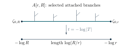
Proposition 4.3.1. NAG-000150 The map is a continuous retraction onto . There is a strong deformation retraction from the identity to which preserves .
Proof. Write for a polynomial, using its Taylor coefficients without division by factorials. For , define a seminorm by This is evaluation at followed by the Gauss norm of radius over , hence multiplicative. Its value on is , so it defines a point of the same annulus. For it is . For , translation by the scalar preserves the radius- Gauss norm, since this scalar has exactly that size; hence the point is .
For a skeletal point , each Taylor term has size at most , while the term already has that size. Thus the homotopy fixes . Finally the displayed formula is continuous in for every polynomial. Inversion of is continuous on the annulus, and Laurent polynomial approximations converge uniformly in its affinoid norm. Therefore all analytic evaluations are continuous along the homotopy. This proves the strong deformation retraction. ◻
The same formula restricts to open annuli because it preserves . This proof also explains what a retraction forgets: the seminorms of individual functions can change along a fibre of , even though the radius is fixed. A function factors through only when it is constant on those fibres.
4.4 Units on annuli and integral slopes
Proposition 4.4.1. NAG-000152 For a nonzero analytic function on a closed annulus, its skeletal function is It is piecewise affine with integral slopes. If is an analytic unit on the annulus, is affine.
Proof. The formula is the Gauss norm. Uniform convergence of the Laurent series and the positive minimum of its Gauss norm on the compact radius interval show that only finitely many terms can attain the minimum. Thus is the minimum of finitely many affine functions with integral slopes. In logarithmic radius , the function is convex. If has an inverse, multiplicativity gives , and this negative is convex as well. Therefore , and hence , is affine. ◻
Example 4.4.2. For with , one has . The slope drops by one when the radial path passes the radius of the zero. On the full analytic curve, a branch toward is attached there; along that branch increases with slope one. The additional branch restores the zero total outgoing slope at the nonclassical attachment point. Looking only at the interval would lose this contribution.
A monomial map sends the skeletal coordinate to and multiplies lengths by . Its injectivity on an interval does not make it unimodular: the tangent-lattice index is . This distinction will reappear in tropical multiplicities and faithful tropicalization.
4.5 Residual curves and tangent directions
Let be a smooth proper connected algebraic curve over . At a type II point , the field is a one-variable function field over . Let be its smooth projective curve. A tangent direction at is a germ of a nontrivial path leaving ; equivalently it is a branch in a sufficiently small suitable neighborhood.
NAG-900005 Proof review pending
Theorem 4.5.1. There is a canonical bijection at a type II point. A type III point has two directions, and a type IV point has one. In a semistable model containing as a vertex, is the smooth normalization of the residual component attached to ; nodes determine distinguished directions.
Proof. Write . By [StacksAlg] (Tag 0A26) the proper curve is projective. The empty-marking case of Theorem 4.38.2 gives a projective split nodal model with the specified generic fibre. By Theorem 4.13.2 the analytic generic fibre of its completion is . Given a type II point , apply Theorem 4.27.4 to . On the resulting model Theorem 4.29.2 identifies the normalization of the component at by its function field , and identifies its closed points with the intrinsic branches at , independently of the model. The normal proper curve with this function field is its nonsingular projective model, which is smooth because is perfect [StacksAlg] (Tag 0BY3). Its closed points are -rational because is algebraically closed. On a model containing the cofinal punctured stars of Theorem 4.25.3 identify the two ends of a self-node with distinct normalization points.
For the remaining valences use the open disc and open annulus tubes of Theorem 4.23.3. Their complement consists of type II component points. Each tube is an open subspace of an analytic line in its chart, so it suffices to count local branches there. Use the disc classification of Theorem 4.1.1. At a type III point , . The circle consists of : the nonzero monomials in each polynomial in have distinct norms, since is divisible. Open annuli with radii straddling are cofinal neighbourhoods. Indeed finitely many polynomial evaluations determine a basic neighbourhood, and after factoring those polynomials the absolute values of their linear factors near this circle are either constant or equal to . Each punctured annulus has precisely two components, its inner and outer open annuli. Each is path connected by the radial homotopy of Proposition 4.3.1; shrinking preserves the two labels.
At a type IV point take nested closed discs with empty intersection representing , passing to a subsequence with strictly decreasing radii. Writing the discs as , use the open discs . Each contains and lies inside . Thus these neighbourhoods of are cofinal: eventually the discs exclude all the roots of any given finite list of nonzero polynomials, so those polynomial norms are constant on the disc. Each such open disc remains path connected on deleting . Indeed any two other points in it can be enlarged to the same closed disc strictly inside it, centred at its centre, with radius larger than both values of the centred coordinate. Along either enlargement the point is the starting point or a disc point with a centre in : for a nested-disc point an enlargement exceeding its limiting radius contains a member of the defining sequence and is centred there. Thus neither path passes through . These continuous enlargement paths are the disc homotopy of Proposition 4.21.2 in a disc coordinate, or equivalently the Gauss enlargement of Proposition 4.3.1. The punctured neighbourhoods are nonempty and give one branch.
It remains to check the model assertion when the supplied model is an arbitrary admissible semistable formal model of . Return to a component vertex on this model and write for the generic point of its component, , and . We use only that the special fibre is a reduced nodal curve and that the generic fibre is the given analytic curve. The following collars are taken on the split algebraic model realizing , which we call the reference model.
On an affine formal chart containing , the prime of the reduction defined by is the minimal prime of . Proposition 4.12.2 gives the unique point over ; Proposition 4.24.2 identifies the fraction field of the reduced chart component with by evaluation. Restriction to a smaller chart gives the same map on the function field, so canonically.
We verify completeness of the normalized component without a properness assumption on an individual affine chart. Apply Theorem 3.19.25 at with the whole quasi-compact quasi-separated strictly analytic curve as neighbourhood, first with and then with the completed reference model. It identifies the two spaces of valuations with centre on the respective reduced components, over the space of valuations of . Here the reduced closure in each application is exactly the indicated component. The reference component is proper, so every valuation of has exactly one centre on it, by the valuative criterion for properness [StacksAlg] (Tag 0BX5, (1) to (3)). Consequently every such valuation has exactly one centre on . Its normalization is finite and birational [StacksAlg] (Tag 0BXR, (1) and (3)), hence proper [StacksAlg] (Tag 02OG, (1) to (2)), since is locally noetherian. Lemma 3.19.23 applied to thus gives exactly one centre on as well.
For clarity, this centre comparison identifies with the smooth projective curve , over . At a closed point of either normal curve the local ring is a DVR [StacksAlg] (Tag 00PD, (5) to (1)). A nontrivial valuation ring of dominating this DVR equals it: a uniformizer has positive value and every element of is a unit times a power of that uniformizer. Each such valuation has a unique centre on each curve, and the centre cannot be generic. Thus the identification by valuations matches the closed points and their local rings inside . Both curves are integral noetherian curves of finite type over ; their proper closed subsets are finite sets of closed points. This gives a homeomorphism, including the generic point. On any nonempty open of an integral scheme, the regular functions are the intersection of its local rings in its function field (the local representatives agree on overlaps). The homeomorphism therefore gives the unique isomorphism inducing the identity on . Denote the normalization map by .
We now show that the branch indexed by actually specializes to near on . Choose a finite formal affine cover of , as in the proof of Theorem 3.19.25. The affinoid generic fibres are compact in the Hausdorff curve. Near we can discard the finitely many which miss . For each remaining chart , lift finitely many -algebra generators of to . Write for their images on the reduced component. Choose representing at , taking if . For this choice, write each nonzero on an affine open of the reference component as a quotient of residues of two functions on a reference algebraic model affine, with nonzero denominator at the component generic point. Lifting that quotient gives of norm one at . On a dense open of the reference component the numerator and denominator are regular and the denominator has nonzero reduction. There is a regular model function after inverting the denominator. The functions are analytic on an ordinary neighbourhood of : its algebraic support is generic since a closed point of is -rational and cannot have type II. Continuity on now gives A single ordinary neighbourhood works on the corresponding chart intersections for all members of the finite list.
For a nonzero rational germ of norm one at , the reference branch collar with coordinate , , satisfies Indeed is a unit on a neighbourhood of ; cofinality of the reference stars puts the whole thin collar there. Theorem 4.24.5 gives the formula on the Gauss segment and Corollary 4.10.3 extends it to all points of the collar.
Fix and a chart . If lies outside its special affine, some nonzero has a pole at : otherwise the coordinate ring of the affine piece of , generated by the , lies in . This would give the same valuation a centre in the affine piece, contrary to uniqueness. For this , on the thin collar, which excludes there by and . If lies in the special affine, lift the values to . When vanishes in , near by continuity. Otherwise its order at is positive, so the collar formula gives on the thin collar. Consequently there on for every . These inequalities cut out the tube of the single closed point in this chart, since the reduced coordinate values of the generators determine the point. Finiteness of the cover gives the claim on a whole collar of the branch.
Finally the cofinal stars can respect these specializations simultaneously. Remove from the finitely many reference node branches, the complements of the preimages of the special affines just used, and the complements of the dense smooth reference opens on which all are regular model functions with the specified reductions. These exceptions are finite since each of the chosen opens contains the component generic point. For a remaining , throughout its reference tube the reduction of is its value : in a model affine reduces to zero at the specialization. Hence within the common ordinary neighbourhood from above, every point of that tube reduces on to , in whichever chart contains it. Take a reference star contained in this neighbourhood and in any prescribed neighbourhood of , and thin its finitely many exceptional branches by the preceding collar argument. Theorem 4.25.3 supplies such stars with connected punctured pieces. Each piece is now in the formal tube of its specified point. Lemma 4.24.1 on the reduced nodal special fibre identifies the points above a node with its two geometric branches (the residue field is algebraically closed). At a self-node these are distinct points of this same ; their punctured-star pieces are disjoint even though both specialize to that node. ◻
For the Gauss point on , : the finite residual points give the inward discs and the point at infinity gives the outward branch. On the closed unit disc, that outward branch is absent from the domain. On a general curve the residual curve can have positive genus. Replacing it by would discard precisely the geometry that residual degree and harmonicity can detect.
4.6 Semistable vertex sets and formal models
Definition 4.6.1. A semistable vertex set of is a finite set of type II points such that is a disjoint union of open balls and finitely many open annuli. Its skeleton is together with the skeleta of those annuli. The length of an annular edge is its logarithmic modulus.
NAG-900006 Proof review pending
Theorem 4.6.2. A smooth proper connected curve over the specified algebraically closed complete field has semistable vertex sets. Semistable formal models correspond to such vertex sets. A model dominates another exactly when its vertex set contains the other one. The associated finite metric graph is a skeleton of the analytic curve, and the local retractions glue to a deformation retraction onto it.
Proof. Let , , and choose with . Write for the given smooth proper connected curve and . The curve is projective [StacksAlg] (Tag 0A26). Fix any admissible semistable formal model with its identification . We will apply the correspondence for algebraic completions by proving that this very model is such a completion over . Its special fibre is a reduced curve with at worst nodes. No pointed chart on is a hypothesis of the argument.
The formal model has a finite cover by formal affines: apply the finite chart argument in Theorem 3.19.25 to the whole compact strictly analytic curve. Their generic fibres form an analytic covering with the neighbourhood property, and specialization is surjective. Hence is of finite type over . For every irreducible component its generic point has a unique analytic lift by Proposition 4.12.2; this is a type II point by Proposition 4.24.2. The formal-model clause of Theorem 4.5.1 identifies the normalization of that component with its smooth projective residual curve. Thus the disjoint union of the normalizations is proper over , and is finite surjective by [StacksAlg] (Tag 0BXR) (or Lemma 4.24.1). In particular is proper. Indeed, after any base change the preimage of a closed subset of under this surjection has the same image in the base as the closed subset, so is universally closed. The finite morphism maps the closed diagonal of onto the image of the diagonal of . The latter image is closed. The diagonal is a closed immersion locally around its image, on for affine opens ; it is therefore a closed immersion. This proves separatedness as well.
Put and let be the -th scheme truncation of , for . These form a cartesian tower, with . The ideal is nil since has rank one. Its extension to any ring is nil, so passage to the closed fibre gives a homeomorphism also after any base change on , for the base, the source and its fibre square. Universal closedness for follows from that for after these identifications. The diagonal image of is likewise closed. The same affine diagonal argument over gives separatedness.
On a formal affine admissibility gives a surjection and -torsion-freeness. Every nonzero element of divides some , so is -torsion-free, hence flat [StacksAlg] (Tag 0539). Thus is flat over . It is a quotient of , because a restricted series reduces to a polynomial. To check finite presentation, apply [StacksAlg] (Tag 05IK) on to the cyclic -module . The polynomial morphism is finitely presented, the module sheaf is of finite type, and the base has only one point, so its weakly associated points are locally finite. Every stalk of this sheaf is -flat: localization is a filtered colimit of copies of the flat module . The theorem gives finite presentation on the entire affine space. Consequently the kernel of is finitely generated, and is a finitely presented -algebra. The finite affine cover and separatedness now give properness, flatness and finite presentation of every .
Proposition B.1.2 and Theorem B.1.3 apply to precisely this tower. They give a projective flat finitely presented -scheme , at worst nodal of relative dimension one, together with compatible isomorphisms at all levels. On formal affines the rings and their restriction sheaves are the -adic inverse limits of those truncations. We obtain an isomorphism and, by Theorem 4.13.2, the specified analytic isomorphism .
This last identification comes from an isomorphism . Here is the precise use of Theorem 2.34.8. For projective -schemes , embed in projective space. An analytic map pulls back the hyperplane line bundle and its generating sections. The theorem algebraizes the line bundle and the sections; the evaluation map is surjective because its coherent cokernel has zero analytification. They define a map to projective space [StacksAlg] (Tag 01NE). Its analytification is the original projective-space map, as one sees on each coordinate chart by taking ratios of the sections. Each homogeneous equation of pulls back to an algebraic section of a tensor power whose analytification vanishes, hence to zero. The map therefore factors through scheme-theoretically. Two such algebraic maps with the same analytification have isomorphic bundles with the same ordered sections by full faithfulness, so are equal. Applying this argument to the isomorphism and its inverse gives the assertion, with the prescribed identification.
In particular is smooth. Theorem 4.18.2 gives split pointed charts at the finitely many special nodes: its finite extension is , and smoothness of makes every smoothing parameter nonzero by Theorem 4.15.3. Smooth closed special points have residue field , which is algebraically closed. Thus , with its generic identification, is a split nodal algebraic model of . The formal isomorphism over identifies the specialization maps and the component vertices.
Theorem 4.38.2, with no markings, supplies an initial model. Theorem 4.42.5 now applies to every model under consideration: it realizes every semistable vertex set, identifies the arrows inducing the identity on with reverse inclusions, and identifies the graph with its original logarithmic edge lengths. The local disc and annulus retractions glue by Theorem 4.23.3; transport along the formal isomorphism gives the asserted deformation retraction. ◻
The special fibre explains the gluing. Tubes of smooth closed points are open balls; tubes of ordinary double points are open annuli; generic points of components lift to the vertices. The annular modulus comes from an equation , and the incidence of components gives the incidence of edges. This reconstructs a metric graph from a model, while Theorem 4.6.2 supplies the converse construction.
Adding a type II point in an annular edge subdivides the edge without changing its total length. Adding a vertex in a ball attaches a new tree segment. The skeleton therefore depends on the chosen model, although the metric on common paths is compatible. For punctured curves, one chooses a vertex set compatible with the finitely many punctures and adds the corresponding infinite rays. Over a non-algebraically-closed field, semistable reduction can require a finite extension; descent of models, weights and integrals must then be handled separately.
4.7 The slope formula and its sign
Let and put away from its zeros and poles. At a type II point , choose with . The residue of is a nonzero rational function on , defined up to a nonzero residual constant. Its divisor is therefore unambiguous.
NAG-900007 Open proof obligation
Theorem 4.7.1. (Slope formula). For a direction at a type II point, corresponding to , Only finitely many slopes are nonzero, and their sum is zero. On a skeleton of the punctured curve containing all zeros and poles among its ends, factors through the retraction and is piecewise affine with integral slopes. Toward a zero or pole , with ray parameter for a local parameter , it has slope .
Open proof obligation (RC2). Prove equality of residual orders and analytic slopes in the stated scope; BPRStructure Theorem 5.15 supplies it.
Example 4.7.2. Take at the unit Gauss point of . Its residual function is , with divisor . The outgoing slopes of are toward the residual zero, toward infinity, and zero in all other directions. For , both signs reverse. The later identity uses the latter logarithm; graph Laplacian conventions must be matched to it, rather than inferred from the word “slope”.
4.8 Higher-dimensional skeleta and tropical coordinates
The curve construction has a higher-dimensional local model, but existence of such a model is an additional hypothesis. Suppose a formal model is strictly semistable, with local ètale charts over Its standard skeleton has coordinates with . The Gauss-point construction and residue calculation were given in Section 3.8. The simplex has real dimension , while the generic fibre has analytic dimension .
Definition 4.8.1. (Formal strictly semistable pair). In the setting of [GRW16] (Definition 3.7), take a connected quasi-compact admissible formal scheme with the local charts above, together with distinguished effective Cartier divisors . Each has irreducible support on the generic fibre and, in each chart, is either absent or defined by one of the free coordinates . Their sum gives a formal strictly semistable pair . The irreducibility condition excludes self-intersections of an individual horizontal component.
When horizontal coordinates vanish on the stratum under consideration, the corresponding canonical polyhedron is The unbounded coordinates are on the complement of the horizontal divisor. The remaining free coordinates have Gauss radius one. Thus the polyhedron has dimension , while the associated residual stratum has dimension . Both enter a higher-dimensional slope formula.
Strata index the canonical polyhedra, and their incidence determines the gluing. Writing , GRW constructs the skeleton in and its canonical retraction; see [GRW16] (§§3–5, especially Theorem 4.13). This is an external geometric theorem, extending the explicit annulus construction. The availability of the local equation does not establish a global strictly semistable model for every variety. Alterations and extensions, when used to obtain models, require their own descent arguments.
Definition 4.8.2. On an analytic domain , invertible analytic functions define an analytic moment map and its tropicalization This map need not be injective or have image of the same dimension as . Its coordinates present real functions; the analytic geometry supplies the weights and the admissible local dimensions.
We now pass from this analytic foundation to tropical geometry. Three constructions must be kept distinct: a skeleton attached to a model, the tropical image of a chosen moment map, and the tropical skeleton selected by Shilov points of tropical fibres. GRW relates them under precise hypotheses; the relations, degree formulas and faithful embeddings are developed in Chapter 6. Their differential applications start only after the lattice multiplicities and refinement rules of Chapter 5 have been established.
4.9 Finite Galois descent of the analytic topology
Fix a complete non-Archimedean field with its given absolute value, and a finite Galois extension with group . Give the unique extending absolute value of Lemma 1.12.1. We use the scalar extension constructed in Theorem 2.40.12. The action of on is semilinear over and fixes its projection .
Lemma 4.9.1. NAG-002023 (Galois action on completed fibres). For a -analytic space and , the fibre is a nonempty finite -orbit. More precisely, putting , there is a finite product decomposition where the are finite field extensions of , equipped with their unique extending absolute values. The factors correspond to the points of the fibre, with . The -action permutes the factors transitively and preserves their valued-field structures.
Proof. Choose a -basis of . Its coordinate maps are bounded by Lemma 1.12.1. Tensoring these finitely many maps with compares the projective tensor norm with a coordinate maximum norm on in both directions. The latter is complete. Thus the algebraic tensor is already complete and is the displayed completed tensor.
For a -affinoid algebra , the same coordinate comparison identifies with the finite free -algebra in its canonical finite-module topology. It is -affinoid by Theorem 2.33.18. Every bounded -point restricts on to its unique extending absolute value, so its -spectrum and -spectrum agree. The affinoid fibre formula therefore applies to the projection and gives precisely . These identifications glue on the chart atlas.
By the primitive-element lemma, [StacksAlg] (Tag 030N), write with separable minimal polynomial . The coprimality of and persists in by the same polynomial Bezout identity. Factoring into distinct monic irreducibles over and applying the Chinese remainder construction gives the product of fields . The sum of their degrees is . Each field is complete and has precisely one extending absolute value by Lemma 1.12.1. The fibre construction of Theorem 2.40.13 now gives the point and completed-residue-field assertions.
The fixed algebra is . Indeed, write an invariant element as , with the finitely many linearly independent over . Applying each shows that every lies in , where the last equality is [StacksAlg] (Tag 09DW). If the primitive idempotents of the product had two or more -orbits, the sum of the idempotents in one orbit would be a nontrivial idempotent in this fixed field. This is impossible. Hence the action is transitive. An induced -isomorphism between two factors preserves their absolute values by uniqueness, which completes the proof. ◻
Theorem 4.9.2. NAG-002024 (The scalar-extension quotient). For every -analytic space , the scalar-extension projection is a continuous, open, closed surjection and induces a homeomorphism For every -invariant subset , its induced map is also a homeomorphism, with the subspace topologies. For every topological space , the map is an open quotient map.
Proof. On an affinoid chart , its inverse image is . The field automorphisms of are isometries, so their coefficient actions extend to bounded algebra automorphisms and hence continuous maps of . These actions agree on overlaps and give a continuous -action on . By Lemma 4.9.1, the projection is surjective and its fibres are exactly the orbits.
We verify closedness using the affinoid quasi-net atlas. Let be closed in . For each affinoid chart , the set is closed in the compact space ; its image is compact and thus closed in the Hausdorff space . The quasi-net condition now makes closed in . To see this directly, for choose finitely many chart members containing whose union contains a neighborhood of . Each relative open complement contains , so it contains for an ambient open neighborhood of . The neighborhood is disjoint from . This argument does not require itself to be Hausdorff or good.
A closed continuous surjection is a quotient map. Since its fibres are the -orbits, it gives the stated homeomorphism. It is open as well: for any open , the set is open, so is open by the quotient property.
A -invariant subset is saturated for . If is relatively closed, write with closed in . Saturation gives , which is relatively closed. Thus is a quotient map with orbit fibres and yields the second homeomorphism. Finally, sends a basic open product to the open product . It is a continuous open surjection and therefore a quotient map. ◻
Corollary 4.9.3. NAG-002025 (Descent of equivariant retractions). Let be -invariant and let be a continuous -equivariant strong deformation retraction onto . There is a unique continuous strong deformation retraction onto such that Writing and , a continuous function satisfies if and only if .
Proof. Equivariance makes constant on every fibre of . The quotient property in Theorem 4.9.2 produces a unique continuous . Its value at is the identity, its value at lies in , and it fixes every point of throughout the homotopy: choose a lift in and use the same assertions for . Finally and surjectivity of prove the equivalence for . ◻
For an analytic unit on a -analytic domain , apply the corollary with and an equivariant strong deformation retraction of . Its scalar extension satisfies by evaluation, so the last assertion applies to on . All absolute values here are the fixed original absolute value and its extensions; the logarithmic values are unchanged by descent.
4.10 Laurent coefficients and local slopes
Let be a complete non-Archimedean field, with arbitrary characteristic and possibly trivial absolute value. For , put The coefficient description and its multiplication are supplied by Theorem 2.13.2 and Proposition 2.13.3. For , write and For , the maximum is positive and attained, and the set of maximizing exponents is finite. Denote its least and greatest elements by and , respectively.
Lemma 4.10.1. NAG-002026 (Extreme Laurent exponents). For and , If and , the one-sided derivatives satisfy
Proof. Write and , and fix . The weighted coefficient families tend to zero in both directions. In the coefficient of , the product is the unique summand of weighted size . Indeed, a summand of that size must use a maximizing exponent of each factor, and neither exponent can be smaller than the corresponding minimum. All other summands have strictly smaller size. Their sizes tend to zero, so their supremum is strictly smaller as well. The ultrametric inequality therefore gives a coefficient of that weighted size.
For a smaller exponent, every convolution summand has strictly smaller weighted size, and the same finite-tail argument applies. Gauss multiplicativity, Proposition 1.2.2, now gives the first formula. Choosing the greatest maximizing exponents gives the second formula.
By Proposition 4.4.1, is the minimum of finitely many affine functions on the compact parameter interval. Near , only those attaining the minimum at can contribute. To the right their smallest slope is selected; to the left their greatest slope is selected. This proves both derivative formulas. ◻
Proposition 4.10.2. NAG-002027 (Annular units). An element is a unit if and only if The exponent is unique, and may be taken to be the coefficient of . At every analytic point of the annulus,
Proof. Suppose . Lemma 4.10.1 gives, at every radius, Both terms are nonnegative integers, so has a unique maximizing exponent at every radius. Only finitely many exponents can maximize anywhere on , as in the proof of Proposition 4.4.1. A unique maximizer is therefore locally constant in the radius. Connectedness of gives one exponent throughout; the same conclusion is immediate if .
Set and . At either endpoint every coefficient term of has size strictly less than one. The terms tend to zero, so their maximum is strictly less than one. The coefficient norm is the maximum of the two endpoint Gauss norms; hence . Conversely, Lemma 1.1.4 inverts , so the displayed form is a unit.
For any analytic point, Lemma 1.6.1 gives , whence . This proves the norm identity. Any displayed form has as its unique maximizing exponent at every radius, which proves uniqueness. ◻
Corollary 4.10.3. NAG-002028 (Units on standard open domains). An analytic unit on a standard open annulus , where , has Thus its absolute value factors through the radial retraction. An analytic unit on a standard open or closed disc of positive radius with centre has constant absolute value .
Proof. Restrict an annular unit and its inverse to closed subannuli of positive modulus. Proposition 4.10.2 applies to each restriction. When two radius intervals overlap in a nonempty open interval, the affine functions agree there, so their slope and constant agree. Any two compact radius intervals lie in a common larger compact subinterval of ; comparing with that subinterval gives the asserted global formula.
For a closed disc of radius , translate the centre to zero and write and its inverse . Restriction to the radius- circle identifies these coefficient series with elements of . Their greatest maximizing exponents are nonnegative and sum to zero by Lemma 4.10.1. Both are zero. Consequently and , which gives throughout the disc. Restricting an open-disc unit to each closed subdisc centred at proves the open-disc assertion. ◻
Proposition 4.10.4. NAG-002029 (Residual orders along Gauss-circle paths). Let , let with , and choose with and . Put and Then is a nonzero Laurent polynomial representing the residue of in . For sufficiently small , consider the paths They start at , and For and , the stronger identity holds for all sufficiently small . The path germ is independent of the lift . These statements also apply to a quotient of two nonzero elements of by subtracting their formulas. If is algebraically closed, the sum of the displayed outgoing slopes is zero.
Proof. The coefficients have size at most one, tend to zero in both directions, and at least one has size one. Hence only finitely many have nonzero reduction, and . Such a exists because a maximizing term has size . Laurent polynomials are dense in for a norm dominating , so is the completion of the Gauss-valued field . In the coordinate , Proposition 3.8.1 therefore identifies its residue field with . Laurent truncation leaves a tail of norm less than one, proving that the residue of is exactly .
Its orders at zero and infinity are and . The corresponding path formulas follow from the two one-sided derivatives in Lemma 4.10.1; the outward path changes to .
Fix and a lift , so . For every , substitution of on the closed disc gives Here is the integer binomial coefficient, also for negative . Its absolute value in is at most one. The inner sum converges by Lemma 1.1.2. Moreover the double family of terms has norm at most ; for each positive threshold only finitely many pairs exceed it. The same summability lemma therefore permits the interchange of sums. The negative-power expansion follows by the geometric inverse for , or equivalently by the integer binomial identity. Thus this is an equality of convergent series, and .
Reducing each coefficient identifies with the formal expansion of . If , then and for . Choose so that For , the th term has Gauss size . Each lower term has smaller size by this choice, and each higher term has size at most . Therefore the Gauss norm is exactly . Taking gives the asserted equality and derivative; at the equality is .
If is another lift of , then . For close enough to one, translation by preserves the radius- Gauss norm, so the two path germs agree. For a quotient, both numerator and denominator have positive Gauss value and the established formulas hold on a common short initial segment; subtracting logarithms proves the assertion. Finally, writing If is algebraically closed, the orders of at its nonzero roots sum to its degree. Adding the orders at zero and infinity gives zero. This proves the slope sum, and subtraction gives the same conclusion for quotients. ◻
All coefficient and Gauss-norm calculations above are unchanged by a complete valued extension of that preserves its absolute value. At a radius already in , the initial Laurent polynomial is carried to the extended residue field coefficientwise, so the same path calculation applies there.
4.11 Implicit functions on entire tubes
The simple-root argument of Lemma 2.54.1 extends to a square system of restricted power series and can be made uniform on increasing affinoid domains. We use its contraction construction and the geometric inversion of Lemma 1.1.4, with the maximum norm for vectors and matrices.
Proposition 4.11.1. NAG-002033 (A uniform implicit-function domain). Let be a -affinoid algebra over a complete non-Archimedean field, with an admissible submultiplicative Banach norm. Let , let have coefficients of norm at most one, and fix . Write and put Give the following subsets their analytic-domain structures: Then is an analytic isomorphism. Its inverse has -coordinate equal to the unique vector of analytic functions on satisfying and at every .
Proof. Translation by is a contractive endomorphism of the unit Tate algebra. Indeed, expand each monomial by the integer binomial formula. Its coefficients have norm at most the norm of the original coefficient. For any positive threshold, only finitely many original coefficients exceed that threshold, and each associated monomial has finitely many terms. The series criterion 1.1.2 therefore permits the sums to be interchanged and gives a restricted series with the same bound. Termwise differentiation is also bounded, since integer coefficients have absolute value at most one. Consequently The coefficients of each displayed series tend to zero. In particular all entries of , its adjugate, and have norm at most one.
The equation defines the Laurent affinoid domain , because . The set is open in , and is open in ; domain calculus and base change, Proposition 2.40.5, give their analytic structures. For , put In the defining quotient norm, the original coefficients and have norm at most one, , and by the adjugate formula. These domains cover admissibly: every point lies in the relative interior of some , by choosing .
For vectors with norms at most , telescoping each monomial gives The same bounds pass to restricted series by convergence. Thus preserves the closed radius- ball in and has contraction constant . The iteration from zero used in Lemma 2.54.1 gives a fixed point with . Set ; then and The matrix geometric inverse gives of norm at most one. Its determinant therefore has norm at most one. Hence and define a bounded map and an analytic section .
For later use, the monomial telescoping also gives a matrix difference identity whenever both norms are less than one. Each entry of the remainder contains a monomial of positive degree in ; the restricted-series tails converge, so this is an identity in the Banach algebra, not only at its analytic points.
If , the defining presentations give a contractive restriction . Apply the difference identity to and the restricted . The factor is invertible, since . Hence the roots agree. Analytic morphism gluing gives a section .
We check the other inverse identity on analytic functions. The domains of defined by and , for , form an admissible affinoid cover. In their defining quotient norms, and the pulled-back has norm at most . The difference identity becomes Thus in the affinoid algebra, and identifies the coordinate as well. The base coordinates already agree, so is the identity as an analytic morphism. The argument preserves nilpotents.
Finally, let be another analytic solution with the stated strict bound. On , restrict further to the Weierstrass domains , where . As and vary, these domains cover admissibly. Their defining quotient norms make the map from contractive and give ; thus all the restricted series substitutions converge. The same difference identity has an invertible matrix factor, since its error has norm at most . It follows in each domain algebra that , and sheaf gluing proves uniqueness on . ◻
Corollary 4.11.2. NAG-002034 (Pointed Jacobian charts preserve entire tubes). Let be nontrivially valued, put and , and let and be admissible formal -schemes with Let and satisfy and . Let be the point over with and . The generic-fibre map induces a canonical analytic isomorphism The same conclusion holds for a finite composition of such pointed charts and for formal-open restrictions containing the chosen special-fibre points.
Proof. Proposition 3.14.7 gives the generic affinoid algebras and their quotient norms. The coefficients of each have norm at most one and tend to zero in this norm, because they lie in and tend to zero -adically. By Proposition 3.20.1, a point of satisfies and . This tube therefore lies in .
Over this base tube, specialization to is equivalent to . The base coordinates already specialize to , these inequalities fix the residues of all , and forces the specified residue of . These coordinates generate the special-fibre algebra and hence determine its specialization point. Thus Restricting the preceding isomorphism proves the assertion. Two lifts of differ coordinatewise by elements of and define the same strict inequalities; the unique inverse is consequently independent of the lift. A formal open containing contains its entire tube in the generic fibre. Indeed, the principal-open specialization criterion applies to a principal neighborhood of inside that formal open. Formal-open restrictions therefore preserve the isomorphism, and composition gives the final assertion. ◻
4.12 Reduced models and component points
Let be complete and nontrivially valued, with its original absolute value. Put , , and . Fix .
Lemma 4.12.1. NAG-002035 (A reduced special fibre determines the unit ball). Let be an admissible -algebra, let , and assume that is reduced. Then the quotient norm associated to any admissible integral presentation of is power-multiplicative and equals the spectral radius. Moreover, In particular, both and are reduced.
Proof. Use Proposition 3.14.7, including the norm-attaining lifts in its proof. It identifies with the quotient closed unit ball. For nonzero , its norm is attained by a restricted power-series lift, whose nonzero norm is the maximum of its coefficient absolute values. Thus . It follows that One inclusion follows from the ultrametric inequality for finite sums. For the other, choose with ; then . The case is immediate.
For any nonzero , choose with and put . Its class in is nonzero. Reducedness implies that every positive power of this class is nonzero. Since , the displayed characterization of gives for all . Consequently A nonzero nilpotent is incompatible with this identity. Power-bounded elements are exactly those of norm at most one, and topologically nilpotent elements are exactly those of norm less than one. This proves all three identifications. ◻
Proposition 4.12.2. NAG-002036 (The analytic point of a residual component). Let be an admissible formal -scheme with reduced special fibre, and let . For each generic point of an irreducible component of , the fibre consists of a unique point . On each formal affine open, these points are exactly the Shilov boundary of its generic fibre. They agree under restriction to formal opens. If is quasi-compact, the resulting component-point set is finite.
Proof. Choose a formal affine open containing . The preceding lemma identifies its special fibre with strict canonical reduction. Theorem 3.16.7 therefore gives a unique point above each component generic point and identifies these points with the Shilov boundary of .
The specialization and formal-open compatibility in Proposition 3.17.2 give . Thus every global point above already belongs to this affine generic fibre. This proves global uniqueness as well as existence. On two formal affine opens, restriction to an affine open in their intersection containing shows that the constructed points agree.
Finally, a finite formal affine cover exists when is quasi-compact. By Corollary 3.12.5, the generic fibre of each member has a finite Shilov boundary. Every global component generic point lies in a member of the cover, so its analytic lift belongs to one of these finitely many finite boundaries. This proves finiteness. ◻
4.13 Algebraic models and formal completion
Let be a complete nontrivially valued non-Archimedean field with its specified real-valued absolute value. Put and fix with . All completions below are -adic. The value group need not be discrete.
Lemma 4.13.1. NAG-002037 (Affine algebraic models). Let be a finitely presented flat -algebra, with a presentation Its completion is an admissible -algebra, and the natural maps give The generic fibre of is canonically the analytic domain in , with the displayed affinoid algebra. For , the completion of is the principal formal-open algebra Its generic fibre is the domain in the preceding bounded-coordinate domain. These identifications respect the polynomial coordinate maps and their restrictions.
Proof. The completion of is : a compatible polynomial system modulo gives one coefficient in the complete ring at each monomial, and for every only finitely many coefficients survive modulo . Conversely such a restricted coefficient family gives the compatible polynomial system. The powers of define the given topology on .
Apply Lemma 3.14.8 to . It makes surjective, with kernel the closure of from . The ideal is closed by Proposition 3.14.5. Polynomial approximation of the finitely many coefficients in a sum shows that this ideal is exactly the stated closure. This proves the restricted quotient presentation.
Flatness of preserves injectivity of multiplication by on . Hence has no -torsion. Lemma 3.14.8 gives the same assertion for and gives all the reduction isomorphisms. The displayed quotient is topologically of finite type; Theorem 3.14.4 makes it topologically finitely presented, so it is admissible. By Proposition 3.14.7, inverting gives the displayed strict affinoid algebra. Theorem 2.33.23, with all radii equal to one, identifies it with the asserted analytic domain, including its analytic structure.
Localization preserves -flatness. Apply the quotient calculation to to obtain the last presentation. Equivalently, its reductions modulo every are , so it is the principal open restriction of . Proposition 3.17.1 identifies its generic domain by ; every already has absolute value at most one there, giving . All these maps agree on polynomial coordinates and their inverses, hence agree on the completions by continuity. ◻
Theorem 4.13.2. NAG-002038 (Completion of a projective model). Let be a projective, finitely presented, flat -scheme, and let be its -adic formal completion. Then is an admissible formal model of : there is a canonical analytic isomorphism For a closed immersion , the generic fibres of the completed standard affine charts are the domains Their overlap maps are the usual coordinate-ratio maps.
Proof. Choose the indicated projective embedding and write . These are finitely presented flat affine -schemes: flatness and local finite presentation restrict to open subschemes, and each is affine and quasi-compact. Its coordinate algebra is generated by the ratios . A finite-type presentation using these chosen generators has finitely generated kernel. Indeed, if is any finite presentation, express and in ; the finitely many relations and generate the kernel, by substituting in a polynomial relation.
By Lemma 4.13.1, each is admissible. On , the same lemma identifies the completed overlap with the principal formal open of . The reduction formula modulo every identifies these overlaps with the restrictions of . Their inverse limits therefore glue to exactly , proving its admissibility.
The generic fibre of the th completed chart is, by that lemma and Theorem 2.33.26, the actual closed-unit-coordinate domain of , with the same quotient ideal. No reduction of that ideal is taken. The completed overlap adds the bound to , hence gives the domain inside . This is exactly ; the remaining coordinates change by division by . Thus the coordinate identifications agree as bounded affinoid algebra homomorphisms on every overlap.
The domains cover : at any analytic point choose a homogeneous coordinate of maximal absolute value. This is precisely the projective affinoid covering in Proposition 2.33.30. Proposition 3.17.2 constructs the generic fibre by gluing the completed affine charts along the overlaps just identified. The same domains and the same transition maps consequently give the asserted analytic isomorphism. On every chart its map is induced by , so these local maps define the natural comparison map to . Its definition on affine restrictions is independent of the projective embedding, which proves canonicity. ◻
4.14 Stable models over valuation rings
A stable family of genus is a proper, flat, finitely presented family of curves whose geometric fibres are connected nodal curves of genus with ample dualizing sheaf. This is the stable-family convention of [StacksAlg] (Tags 0E75, 0E76, 0E78). A stable model of a smooth projective curve over a valuation ring includes an identification of its generic fibre with . We first obtain a finite extension of the fraction field by taking a closed point on a proper algebraic-space cover of the moduli stack.
Lemma 4.14.1. NAG-002043 (Finite extensions in the valuative criterion). Let be a valuation ring with fraction field , let be an algebraic stack proper over , and let be an -morphism. There is a finite field extension such that, for every valuation ring dominating and having fraction field , the object extends to an object of . Such valuation rings exist.
Proof. The scheme is quasi-compact and quasi-separated, and is separated and of finite type. Chow’s lemma for algebraic stacks, [StacksAlg] (Tag 0CQ8), gives an algebraic space and a proper surjective morphism . Proper morphisms compose by [StacksAlg] (Tag 0CL7); hence is proper. The compatibility of properness for algebraic spaces and stacks is recorded in [StacksAlg] (Tag 0CL4).
The fibre product is an algebraic space. Indeed, its map to is the base change of the representable diagonal of ; see [StacksAlg] (Tag 04XS). Properness and surjectivity survive this base change, so is a nonempty proper algebraic space of finite type over . Choose a nonempty affine open in an étale scheme presentation of . The morphism is locally of finite type and quasi-compact, so is a finite-type -algebra. A maximal ideal of has residue field finite over by [StacksAlg] (Tag 00FV). The resulting point of gives a point and a specified isomorphism between its image in and .
Fix any valuation ring as in the statement. Apply the ordinary valuative criterion for the proper algebraic space , [StacksAlg] (Tag 0A40), to It supplies a unique extension of . Its composite with , together with the preceding generic isomorphism, is the required extension of . Finally, [StacksAlg] (Tag 00IA) applied to the local subring supplies such an . Domination ensures : if , then , which excludes . ◻
Theorem 4.14.2. NAG-002044 (Stable reduction over a valuation ring). Let be a valuation ring with fraction field , and let be a smooth projective geometrically connected curve of genus . There is a finite field extension such that, for every valuation ring with fraction field extending , the curve has a stable model which is a projective scheme, flat and of finite presentation over . If has rank one, then has rank one.
Proof. The curve gives a -object of the stack of stable curves of genus , by [StacksAlg] (Tags 0E75, 0E78). This stack is proper over : [StacksAlg] (Tag 0E9C) proves properness over , and [StacksAlg] (Tag 0CL6) preserves it under base change. Lemma 4.14.1 therefore gives a finite extension and, over each as stated, a stable family of algebraic spaces whose generic fibre is identified with . As an object of the stack of curves, this family is proper, flat and of finite presentation by [StacksAlg] (Tag 0D4Z).
We verify that this family is a projective scheme. Let be the closed point of . Stability of and [StacksAlg] (Tag 0E74) give an open neighbourhood of on which is relatively ample. Every open neighbourhood of the closed point of a local spectrum is the whole spectrum: a basic open containing that point has a unit. Hence . By [StacksAlg] (Tag 0D32), relative ampleness over the scheme implies that is a scheme. Properness and the ample invertible sheaf make locally projective by [StacksAlg] (Tag 0B5N). Apply the same local-spectrum observation to the projective neighbourhood of ; thus is projective.
For the last assertion, the value group of has finite index in that of by [StacksAlg] (Tag 0ASH). Write the groups additively as . Every element of has a positive integer multiple in . If is a nonzero convex subgroup, multiplying one of its nonzero elements shows that is nonzero and convex in . Rank one of gives . For any positive , some lies in ; convexity then gives . Thus , proving that has rank one. ◻
Corollary 4.14.3. NAG-002045 (Stable models for the fixed absolute value). Let be a complete non-Archimedean field with its given nontrivial absolute value, and let be a smooth projective geometrically connected curve of genus at least two. There is a finite extension , endowed with the unique extending absolute value, for which has a projective stable model over . If , the extension may be chosen Galois.
Proof. Apply Theorem 4.14.2 to . Lemma 1.12.1 supplies the unique extending absolute value on the finite extension ; its valuation ring dominates , and is complete. We may therefore take in that theorem.
If , take a finite normal closure of using [StacksAlg] (Tag 09DT). Every irreducible polynomial over a characteristic-zero field has nonzero derivative and is relatively prime to its derivative, so is separable and hence Galois. Uniqueness of the extended absolute values identifies the restriction from with the chosen value on , giving . Base change of the stable model to remains stable by [StacksAlg] (Tag 0E76), and remains projective, flat and of finite presentation. Replacing by proves the assertion. ◻
Lemma 4.14.4. NAG-002046 (Extension of an isomorphism of stable generic fibres). Let be a valuation ring with fraction field , and let and be stable families of the same genus . Every isomorphism extends uniquely to an -isomorphism .
Proof. The moduli stack is separated by [StacksAlg] (Tag 0E9A). By the definition of separatedness for stacks, [StacksAlg] (Tag 04YW), its diagonal is proper. Pulling this diagonal back by the pair gives the algebraic space the identification with the isomorphism sheaf is the fibre-product description in [StacksAlg] (Tag 04XS). The morphism is proper by base change. A specified generic isomorphism is a -point of . The proper algebraic-space valuative criterion, [StacksAlg] (Tag 0A40), extends it uniquely to an -point of , which is precisely the required isomorphism. ◻
Corollary 4.14.5. NAG-002047 (The semilinear action on a stable model). Let be a complete non-Archimedean field, let be finite Galois with group , and give its unique extending absolute value. Let be a smooth projective geometrically connected curve of genus , and let be a stable model of with its generic-fibre identification. The canonical semilinear -action on extends uniquely to a semilinear -action on . More explicitly, with and , there are unique automorphisms satisfying and inducing the canonical action on the generic fibre.
Proof. Uniqueness in Lemma 1.12.1 gives for every and , so preserves . Our inverse convention gives . The scheme has the corresponding canonical left action induced by .
For a fixed , form , with its structure map given by the second projection. Both this twist and are stable families over . The generic action gives an -isomorphism : its two components are the generic semilinear automorphism and the structure map to . Lemma 4.14.4 extends it uniquely to an -isomorphism . Composing with the first projection defines . Since is an automorphism, that projection is an isomorphism of schemes, and is an automorphism covering .
The maps and cover the same base map and agree on the generic fibre. Reinterpreting them as -isomorphisms , uniqueness in Lemma 4.14.4 makes them equal. The same argument gives and proves uniqueness of the action. ◻
4.15 Pointed nodal charts over the valuation ring
Let be a complete non-Archimedean field with its given nontrivial absolute value. Write , and . We turn the étale base neighbourhood in the nodal normal-form theorem into the spectrum of the valuation ring of a finite extension. The two field-theoretic ingredients are simple-root lifting and a lift of a finite separable residue extension.
Lemma 4.15.1. NAG-002049 (Simple roots over a complete valued field). The valuation ring is henselian. If is étale and lies over the closed point with , then an affine open neighbourhood of admits a section over through . Its image is open in .
Proof. Let have a simple root after reduction, and choose a lift . Then and . Expanding at gives Choose a real number with . On the complete closed ball , the map takes values in the same ball and satisfies Starting with , its iterates satisfy ; the ultrametric inequality makes them Cauchy. Their limit is a fixed point. Thus lifts and satisfies . This is the one-variable contraction used in the proof of Lemma 2.54.1, now applied to a residue root. The simple-root characterization in [StacksAlg] (Tag 04GG) proves that is henselian.
Choose an affine open containing . The map is étale. Part (8) of [StacksAlg] (Tag 04GG) supplies the -algebra retraction whose inverse image of is the prime of . The corresponding section passes through . A section of an unramified morphism is an open immersion by [StacksAlg] (Tag 024T); hence its image is open in and in . ◻
Lemma 4.15.2. NAG-002050 (Lifting a finite separable residue extension). Let be a finite separable extension. There is a finite separable extension , with the unique extending absolute value, and a -isomorphism such that
Proof. By the primitive-element theorem, [StacksAlg] (Tag 030N), write with monic irreducible polynomial of degree . Lift its coefficients to a monic polynomial of degree . Choose a root of in an algebraic extension of , set , and use Lemma 1.12.1 to equip with its complete extending absolute value. Then .
If , the leading term of strictly dominates every other term, which is impossible. Thus , and defines an embedding sending to . The value-group and residue-degree inequality [StacksAlg] (Tag 0ASH) gives All inequalities are equalities. In particular the residue embedding is an isomorphism, the value-group index is one, and is the minimal polynomial of . Since is separable, , so is a unit of . The minimal polynomial is therefore separable. ◻
Theorem 4.15.3. NAG-002051 (A rational pointed nodal chart after finite extension). Let be a morphism of schemes which is at-worst-nodal of relative dimension one, and let be a node of its closed fibre. There are a finite separable extension , an affine -scheme , étale morphisms and a -rational point of the closed fibre of such that its image in lies over and its image in is the origin . The point is a split node, with If the generic fibre is smooth over , the parameter satisfies , and consequently .
Proof. Apply the nodal normal-form theorem [StacksAlg] (Tag 0CBY). It gives étale maps , and and a point mapping to . Let be its image. A nodal point of a curve has finite separable residue field over the ground field by [StacksAlg] (Tag 0C4D). The étale fibre description [StacksAlg] (Tag 02GL) makes finite separable as well. Hence is finite separable over .
Choose by Lemma 4.15.2, with a specified identification . Base change the diagram to . The maps and define a rational point of , whose image in is rational. Replace by an affine open containing and by its inverse image. Since is complete, Lemma 4.15.1 gives a section through . Pull back the diagram along . Its image is open, so the resulting is open in ; in particular remains étale. The other map becomes étale over , where is the pullback of the parameter . These uses of composition and base change are [StacksAlg] (Tags 02GN, 02GO). The point belongs to this pullback because its image is the special point of the section. Choose an affine open neighbourhood of it and denote the point by .
Let and be the images of in and . Both are rational: their residue fields are intermediate fields between and . The point remains a node by the base-change invariance in [StacksAlg] (Tag 0C56). Applying the étale invariance of nodes, [StacksAlg] (Tag 0C57), to the two maps from shows that and are nodes. The curve is smooth wherever or is invertible; its only possible nodal point is therefore . Thus is that origin and .
The local rings at , and of these special fibres are Noetherian, since the fibres are locally of finite type over . Each of the two étale local maps is flat, has the same residue field , and carries the source maximal ideal onto the target maximal ideal; flatness and the fibre assertion follow from [StacksAlg] (Tags 02GS, 02GL). Thus [StacksAlg] (Tag 0AGX) identifies their completions. The completion at is , giving the displayed isomorphism for . The split-node criterion [StacksAlg] (Tag 0CBW) completes this assertion.
Finally assume that is smooth, and suppose . Then has the section over . The image of is open by [StacksAlg] (Tag 03WT) and contains the closed point of this section. Its inverse image on is an open neighbourhood of the closed point, hence the whole local spectrum. In particular the image contains the generic point of the section, the node of . Any point of mapping to this node is itself a node by [StacksAlg] (Tag 0C57). On the other hand is étale and is smooth, so is smooth; preservation of smoothness under étale precomposition is included in [StacksAlg] (Tag 036U). This contradiction proves . Together with it gives . ◻
4.16 Coordinate changes on annuli
Let be a complete non-Archimedean field, with its specified absolute value. We use the Gauss skeleton, radial retraction and strong homotopy of Proposition 4.3.1. The parameter of that homotopy is denoted by .
Theorem 4.16.1. NAG-002030 (Annulus isomorphisms and radial homotopies). Let and , and let be an analytic isomorphism. Write for the coordinates of . There are , and with such that For every , Thus restricts to an isometry of Gauss skeleta for their logarithmic metrics. In coordinates and , this isometry is , where . Moreover, for every and ,
Proof. Put . Proposition 4.10.2, applied to and to the inverse isomorphism, gives with and . The norm identity in that proposition holds at every analytic point. Composing the two identities at a point of radius gives Comparing two distinct radii gives . Hence . Surjectivity of and the existence of the Gauss point at every radius show that maps onto .
We identify the image of each Gauss point. Set , , and take a nonzero Laurent polynomial . For every integer , the geometric inverse and the integer binomial formula give Consequently The exponents are distinct. The Gauss norm of the Laurent polynomial on the right inside the difference is therefore , while the error has strictly smaller norm. Thus . Laurent polynomials are dense in the target affinoid algebra, so bounded multiplicative seminorms agreeing on them agree on the entire algebra. This proves the asserted equality of actual analytic points.
For an arbitrary , the norm formula gives . Combining this with the Gauss-point equality proves . Taking negative logarithms gives the stated affine formula and its preservation of logarithmic distance.
It remains to compare the homotopies for . Work in and put For a Laurent series , its substitution on the disc is To check the convergence, the weighted terms are bounded by . The first factor tends to zero as , and tends to zero as . Above any fixed positive threshold only finitely many pairs remain. Lemma 1.1.2 therefore permits the indicated sums and their interchange. The negative powers use the convergent geometric inverse of . All integer binomial coefficients have absolute value at most one, which gives the displayed bound.
Expand at as The binomial coefficients of have the same bound, so for . The first coefficient satisfies Indeed has absolute value one, and both and have size at most . Hence, in the radius- Tate algebra over , The bound follows termwise from ; the same estimate proves convergence.
For a nonzero polynomial , write over , and put Replacing by changes the resulting polynomial by a series of radius- norm at most . The Gauss norm of is . Consequently The left side is the evaluation of at . This follows from the construction of and the bounded substitution , whose coordinate and inverse have norms and . The right side is the evaluation at ; the induced embedding is isometric and hence preserves the Gauss norm. Thus these two points agree on . Their common nonzero value on gives agreement on Laurent polynomials, and density gives agreement on . This proves the homotopy identity for . At it is the identity map, and at it is the already proved compatibility of the radial retractions. ◻
Corollary 4.16.2. NAG-002031 (The original absolute value and edge length). Isomorphic nondegenerate closed annuli over have equal logarithmic moduli. For the nodal chart the radial edge has length , and this length and the preceding coordinate-change identities are preserved by complete isometric extensions of .
Proof. The two logarithmic radius intervals are related by an affine map of slope , so . Lemma 3.20.3 and Proposition 3.26.1, with in the latter’s notation, identify the nodal generic fibre with . Its length is therefore . A complete isometric field extension leaves the coefficients’ absolute values, the Laurent coefficient norms and unchanged. Base change of an analytic isomorphism is an isomorphism by Theorem 2.40.12; reapplying the theorem over the extended field gives the asserted identities. ◻
4.17 Tubes in algebraic models
Let be complete and nontrivially valued, with , , and a fixed satisfying . For a flat finitely presented -scheme , write for its -adic completion. All tubes below are taken in its formal generic fibre.
Proposition 4.17.1. NAG-002039 (An algebraic pointed étale map preserves the tube). Let be an étale morphism between flat finitely presented -schemes. Let and . The induced generic-fibre morphism restricts to an analytic isomorphism
Proof. Lemma 4.13.1 makes these completions admissible, and is compatible with formal open restriction. A Zariski open containing the selected residual point retains its entire tube. We may therefore replace the source and target by affine neighbourhoods of and .
By the square Jacobian presentation in [StacksAlg] (Tag 02GU), after such shrinking the morphism is given by , where Localize once more at , which is nonzero at . Adjoining its inverse as a variable gives the presentation . Completing the polynomial presentation by Lemma 4.13.1 gives Here quotients are the separated completed quotients; their indicated finite relation ideals are closed by the admissible-presentation result. Choose lifts of the coordinates . They satisfy the hypotheses of Corollary 4.11.2, which supplies the required entire-tube isomorphism, including its analytic structure. The case of no variables is the identity case. All the preceding restrictions preserved the tubes, completing the proof. ◻
Corollary 4.17.2. NAG-002040 (The tube of a rational smooth point). Let be a flat finitely presented -scheme. Suppose that is smooth of relative dimension at . Then is analytically isomorphic to the open unit -dimensional polydisc over .
Proof. By [StacksAlg] (Tag 054L), a Zariski neighbourhood of admits an étale morphism . Its image is a -rational point. Apply the preceding proposition. The completion of is ; its generic fibre is the closed unit polydisc. If lift the coordinates of , the specialization criterion identifies its -tube with for every . Translation by gives the stated open unit polydisc. ◻
Corollary 4.17.3. NAG-002041 (Transport of a split nodal chart). Let and put , with special-fibre origin . Suppose that there is a diagram of flat finitely presented -schemes, with both arrows étale and all selected special-fibre points -rational. Then is an open annulus with coordinate satisfying .
Proof. Apply Proposition 4.17.1 to both arrows. The formal completion of is the standard nodal chart of Proposition 3.26.1. Its origin tube is computed in Proposition 3.20.1: with and , the two inequalities and become . Transport this already established analytic identification along the two tube isomorphisms. ◻
4.18 Simultaneous splitting of finitely many nodes
Let be complete with its specified nontrivial non-Archimedean absolute value, and put and . Every finite extension below carries the unique absolute value extending this one.
Lemma 4.18.1. NAG-002052 (Lifting a finite Galois residue extension). For every finite Galois extension , there is a finite Galois extension and a specified -isomorphism such that The last map is induced by reduction.
Proof. Use the construction in Lemma 4.15.2. Write , let be its monic minimal polynomial of degree , and lift to a monic . That proof constructs , with , , , and . It also proves that is separable and that the value groups are equal. We retain these identifications.
Normality and separability of give the distinct roots of in . Apply the simple-root construction of Lemma 4.15.1 in the complete field to each . It gives a root of with reduction . Distinct reductions make these roots distinct. Thus splits in , and is its splitting field. By [StacksAlg] (Tag 09HU), is normal; it was already separable, so it is Galois.
Every -automorphism of preserves its absolute value by uniqueness in Lemma 1.12.1. It therefore induces a -automorphism of . Each defines a -embedding of into itself. Its image has degree over , so it is an automorphism. On the residue generator it induces . These are precisely the automorphisms of , and a -automorphism of is determined by the image of . The constructed roots exhaust all roots of and have distinct reductions; thus an automorphism inducing the identity on fixes . Reduction is therefore a bijective homomorphism, as claimed. ◻
Theorem 4.18.2. NAG-002053 (All lifts of a finite set of nodes). Let be finitely presented and at-worst-nodal of relative dimension one, and let be a finite set of nodes of . There is a finite Galois extension such that every point of over one of the is a -rational split node. Writing , each such point admits an affine -scheme , a -rational point , and pointed étale maps Here is the special-fibre origin, whose prime ideal is . If is smooth, every resulting parameter satisfies . One may take and by reduction.
Proof. If the node set is empty, take . Otherwise, for each , choose the original pointed normal-form diagram and point used at the beginning of the proof of Theorem 4.15.3. Put and . That proof shows that and are finite separable. Embed these fields compatibly into one separable closure of . Choose primitive generators for the finitely many by [StacksAlg] (Tag 030N), and let be the splitting field of their minimal polynomials. It is finite and normal by [StacksAlg] (Tag 09HU). Its generators are separable, so [StacksAlg] (Tag 09HC) makes it separable as well. Thus is finite Galois and contains every and its normal closure.
Apply Lemma 4.18.1 to obtain with . The points over are the points of , and Indeed, a primitive-element presentation writes the left side as , where splits into distinct linear factors. Evaluation at its roots is invertible by the Lagrange interpolation polynomials. Thus every point over is rational and is indexed by an embedding .
Fix such an embedding. By [StacksAlg] (Tag 0BME, part (2)), it extends to a -automorphism of , since is normal. Restriction to the chosen subfield gives an embedding extending . The map defined by gives a rational point of lying over the selected point indexed by . Its image in the étale base neighbourhood is rational as well.
Now reuse the henselian-section step of the proof of Theorem 4.15.3, with this rational point and the fixed field . Lemma 4.15.1 supplies a section of through the point. Its image is open. Pulling the original diagram back along that section and then taking an affine neighbourhood of the rational point gives exactly the two pointed étale maps displayed in the statement. The remaining local arguments of that theorem apply unchanged: they identify the image in the standard chart with its origin, give , identify the completed special local ring at with , and prove when the generic fibre is smooth. No enlargement of occurs in any of those steps.
There are only finitely many and finitely many embeddings for each . Applying the preceding construction to each one proves the assertion for every lift of every specified node, all over the same . The value-group and Galois assertions were already supplied by the first lemma. ◻
4.19 Coordinate independence on open annuli
Corollary 4.19.1. NAG-002032 (Open annuli and their radial homotopies). Let be a complete non-Archimedean field with its specified absolute value. Let be standard open annuli with coordinates . Their radial strong homotopies are obtained by restricting and gluing the closed-annulus homotopies of Proposition 4.3.1. For any analytic isomorphism , there are and such that In particular, preserves the radial retractions and induces a skeleton isometry for and . When both boundary radii are positive and finite, the logarithmic modulus is invariant under analytic isomorphism.
Proof. Every point of belongs to the ordinary interior of some closed subannulus , with . In the formula of Proposition 4.3.1, the homotopy keeps fixed at every parameter value. Its seminorm formula at a point depends only on that point and , not on the chosen end radii. Consequently the homotopies on closed subannuli agree on overlaps. Their restrictions to the ordinary interiors give a continuous homotopy on . The initial map, final radial retraction, and fixed-point identity on the Gauss skeleton hold on each subannulus, hence on . The same construction applies to .
Apply Corollary 4.10.3 to and . It gives constants and exponents with The second identity may be evaluated at Gauss points of any two distinct radii. Thus , so . Surjectivity and the existence of all Gauss radii show that maps onto .
Fix and let be the increasing interval whose endpoints are and . The norm identities for and its inverse identify the inverse image of with as a set. The universal property of analytic domains, proved in Theorem 2.40.8, restricts both morphisms and their inverse identities to these domains. Hence Theorem 4.16.1 applies to this nondegenerate closed-annulus isomorphism. Its Gauss-point and homotopy identities are the restrictions of the asserted ones: both homotopies preserve their radii and remain in the respective closed subannuli. These subannuli cover , proving all the identities. Negative logarithms give the skeleton isometry; its slope has absolute value one, so finite logarithmic interval lengths are preserved. ◻
4.20 The ends of residual tubes
Throughout this section is complete and nontrivially valued, and . A curve model is a flat finitely presented -scheme whose special fibre is a reduced pure one-dimensional scheme. Its formal generic fibre is assumed Hausdorff. We write for the unique analytic point above a component generic point , as in Proposition 4.12.2.
Lemma 4.20.1. NAG-002054 (Boundary points of a closed-point tube). Let be a closed point of the special fibre of a curve model , and put in . Then is open in , its closure is compact, and
Proof. Choose an affine open containing . Formal-open compatibility in Proposition 3.17.2 puts the entire tube inside the compact affinoid . Since is Hausdorff, is closed in , so is a closed subset of and is compact. On every formal affine chart, the inverse image of the closed residual point , when it is present, is given by finitely many inequalities ; use Proposition 3.20.1 and the Noetherian special fibre. These inverse images are relatively open. The affinoid net topology of Proposition 3.17.2 therefore makes open in .
For , write as a prime of the affine special fibre. If , choose and an integral lift . Then , whereas for every . The relative open set separates from , a contradiction. Thus . In a pure one-dimensional Noetherian scheme the proper generalizations of a closed point are component generic points. Their analytic fibres are the singletons by Proposition 4.12.2. This proves the inclusion. ◻
Lemma 4.20.2. NAG-002055 (Two components in a pointed nodal chart). Let be an étale morphism and let map to the origin. In , the ideals and are the two distinct minimal prime ideals. They identify the two distinct irreducible components of through . Under any étale map from to a reduced curve, their generic points map to component generic points; these two images may coincide.
Proof. The local map from the origin is flat, induces the identity on , and extends the maximal ideal to the maximal ideal. Thus [StacksAlg] (Tag 0AGX) identifies The special-fibre ring is Noetherian. By [StacksAlg] (Tag 00MC), completion is faithfully flat, so and inject into and , respectively. Consequently and are prime. Their extensions to are incomparable, so the original ideals are incomparable. Their intersection is zero because it becomes zero in the displayed completion and is injective. Since , every prime contains or . These are therefore exactly the minimal primes. The prime correspondence for localization identifies them with distinct global components through . Finally, an étale map is flat. Going down for a flat map, [StacksAlg] (Tag 00HS), implies that the contraction of a minimal prime is minimal: any strictly smaller prime would lift below the chosen minimal prime. This proves the last assertion. ◻
Proposition 4.20.3. NAG-002056 (Attaching the two ends of a nodal tube). Let be a curve model and suppose given a pointed étale diagram where is affine and the three selected special-fibre points are -rational. In , put and . Let be the component points of the branches , respectively. Then Every net in whose tends to converges to ; every net whose tends to converges to . For each neighborhood of either endpoint in , a full radial tail of is contained in that neighborhood. The image of in is ; the only possible identification is that of with . The two endpoints map to the component points of the corresponding branches of .
Proof. The entire-tube isomorphisms of Corollary 4.17.3 identify with the annular coordinate. Write and . The given map induces the étale morphism by base change, by [StacksAlg] (Tag 02GO). In particular is of finite type over . The two branch fields are and . The map is injective since in . Tensoring with gives the injective map Indeed, for each prime of over of , the corresponding local map is flat by [StacksAlg] (Tag 02GU(1) and (2)). Localizing the displayed map at thus gives an injection at every prime. By [StacksAlg] (Tag 02GL(2)), each of the two affine fibres is a finite disjoint union of spectra of finite separable extensions of its branch field. Either fibre may be empty. This proves that is reduced.
If is minimal in , its contraction is minimal in . Otherwise the contraction contains an element outside both minimal primes of , by avoidance of these two primes. Such an element is a nonzerodivisor on by the displayed injection. But its image in the nonzero field would be zero, a contradiction. For a minimal over the branch prime , localize at the nonzero elements of . The result is a nonzero domain quotient of the corresponding affine fibre algebra, hence a finite extension of that branch field. It is the fraction field of . Its transcendence degree over is one, so [StacksAlg] (Tag 00P0) gives . Thus the special fibre of is a reduced pure one-dimensional curve. Lemma 4.20.2 gives exactly the two components through . Lemma 4.20.1 gives . At , the reduction of is nonzero, so ; at , the reduction of is nonzero, so and gives .
The affinoid is compact Hausdorff. A net in whose tends to has cluster points in , and continuity of forces every cluster point to be . Compactness then implies convergence to : otherwise a subnet outside a fixed neighborhood would have a cluster point there. The inner end is identical. Applying this to the Gauss points with radii tending to the two endpoints proves that both and belong to . If is a neighborhood of in , the compact set has after replacing by an open subneighborhood. Thus a full outer tail lies in . The minimum of on a compact complement similarly proves the inner-tail assertion.
By Lemma 4.20.2, the two residual generic points map to component generic points of . Functoriality of specialization and uniqueness of component points identify the images of . The image of compact is closed in Hausdorff and contains . Conversely, continuity and density of in put that image inside . The restriction is an isomorphism, and an endpoint cannot map into because its specialization is generic. Consequently only the two endpoints can be identified. ◻
Corollary 4.20.4. NAG-002057 (The complete nodal homotopy). Under the hypotheses of Proposition 4.20.3, the radial homotopy on extends uniquely by fixing the attached component points to a jointly continuous strong deformation retraction of onto a closed edge of length . If the endpoint images coincide, this edge is a circle with two distinct incident half-edges at its vertex. The construction is independent of the chosen pointed nodal chart and annular coordinate.
Proof. First work in of the proposition. The annulus homotopy of Proposition 4.3.1 preserves . The full-tail assertion shows that fixing extends this homotopy continuously at both endpoints, uniformly in its parameter. The resulting map is therefore jointly continuous. The Gauss radius map extends to a continuous injection of into , with endpoints ; compactness identifies its image with a closed interval. The extended homotopy fixes this interval and retracts onto it.
The map is a compact-to-Hausdorff surjection, as is its product with , so both are quotient maps. The only possible identified pair consists of the two fixed endpoints. The homotopy therefore descends to a continuous map on , with all strong-retraction identities unchanged. The quotient of the Gauss interval is an interval or, when its endpoints coincide, a circle. Its logarithmic length is by Corollary 4.16.2. The full homotopy commutes with every open-annulus coordinate change by Theorem 4.19.1; continuity on the dense tube gives the same equality at the ends. This proves independence and retains both half-edges of a loop. ◻
4.21 Canonical contraction of a smooth tube
Lemma 4.21.1. NAG-002058 (The compactification of a rational smooth tube). Let be a point where a curve model is smooth of relative dimension one. If is the unique component generic point specializing to , then This closure is the one-point compactification of . In each open-unit-disc coordinate , the sets form a neighborhood basis of in .
Proof. Corollary 4.17.2 gives the disc isomorphism. Smoothness makes the local ring of the special-fibre curve at a regular one-dimensional local ring, hence a domain; equivalently its completed pointed étale coordinate ring is and faithful flatness of completion gives a unique minimal prime. Thus exactly one component passes through . Lemma 4.20.1 shows that the compact closure can add only . The open unit disc is not compact: the continuous function has supremum and does not attain it, as witnessed by its Gauss points of radii . Therefore the closure must add . A compact Hausdorff space obtained by adjoining one point to an open locally compact space is its one-point compactification: the complements of neighborhoods of the added point are compact subsets of the open space, and conversely every such compact subset is closed in the compactification.
For , the closed subdisc is compact, so its complement in is a neighborhood of . Conversely, every compact subset of has a maximum . These subdiscs are therefore cofinal among compact subsets, proving the asserted neighborhood basis. ◻
Theorem 4.21.2. NAG-002059 (The intrinsic open-disc homotopy). Let be the open unit disc over a complete nontrivially valued field , and let be its one-point compactification. Write There is a jointly continuous strong deformation retraction onto , characterized for and by Every analytic isomorphism of open unit discs, including an isomorphism semilinear for an isometric field automorphism, commutes with this entire parametrized homotopy. The homotopy also commutes with projection under any complete isometric ground-field extension. In particular it gives a coordinate-independent contraction of in Lemma 4.21.1.
Proof. For , evaluate at over and then take the radius- Gauss seminorm. It is multiplicative and has Thus it defines a point of , and at it gives . On a neighborhood of any , choose strictly larger than both and . The displayed formula is continuous on polynomials and remains bounded on the closed radius- disc; uniform polynomial approximation proves continuity for its affinoid algebra. This proves joint continuity on . At , the preceding inequality preserves every tail , uniformly in . As , it also puts all images in for , uniformly in . The neighborhood basis of Lemma 4.21.1, whose one-point-compactification argument applies equally to , proves joint continuity at every remaining point. The strong contraction identities follow from the construction.
We check coordinate independence explicitly. An analytic isomorphism is represented by a power series convergent on every closed disc of radius less than one. Such an expansion follows by restricting to those discs and using uniqueness of Tate coefficients on overlaps. Since on , evaluation at its Gauss points and passage of their radii to give for every and . The inverse has the same coefficient bounds. The derivative identity for the two inverse series at implies : both and the derivative of the inverse at are at most one and their product is one.
Put , and . For , expansion over gives Indeed, ; these sums converge, and for all terms after have norm at most . On the radius- disc, For a polynomial write and put . Replacing by changes its Gauss norm by an error at most when . The Gauss norm of is . Thus These are precisely the polynomial evaluations at and . Points of the open disc are determined by polynomial evaluations, so the two points agree. The identities at follow from the endpoints and the extension of a disc isomorphism to its one-point compactification. An isometric automorphism of the coefficient field preserves all these formulas. Finally, under any complete isometric extension, the formulas agree on the original polynomials by the isometric embedding of completed residue fields. At the added endpoint the projection sends the endpoint to the endpoint; continuity follows also from its preservation of the radial tails. This proves all the claimed compatibilities. ◻
4.22 Smooth tubes with a separable residue field
Lemma 4.22.1. NAG-002060 (The integral algebra of a residue-field lift). Let be finite separable and let be the lift constructed in Lemma 4.15.2: the minimal polynomial of is monic and reduces to the separable minimal polynomial of a generator of . Put . Then For every flat finitely presented -scheme , its formal completion and analytic generic fibre commute with this coefficient extension. On a completed affine algebra the corresponding formulas are If the original special fibre is reduced, so is the extended special fibre. Specialization commutes with the projection, and the inverse image of a closed-point tube is the disjoint union of the tubes of the points above that closed point.
Proof. For a nonzero coefficient vector, divide by a coefficient of largest absolute value. All normalized coefficients lie in , and at least one has nonzero reduction. Linear independence of over makes the reduction of this normalized sum nonzero, hence its absolute value is one. This proves the norm formula. It proves the two integral identifications as well, since membership in the closed or open unit ball is equivalent to that property for every coefficient.
A finite free direct sum commutes with every quotient by and with the inverse limit defining completion. Thus for an affine algebraic chart, completing its base change gives exactly ; Lemma 4.13.1 makes this an admissible model. After inverting , the finite coordinate comparison in the proof of Lemma 4.9.1, which uses only finiteness of , identifies the algebraic tensor with the completed tensor. The displayed special-fibre formula follows from . These constructions respect affine restriction, so they glue.
For completeness, separability preserves the required reducedness directly. A reduced finite-type -algebra injects into the finite product of the fraction fields of its minimal-prime quotients. Tensoring with , which is flat over , preserves this injection. Each field tensor with is reduced: remains relatively prime to its derivative and hence factors into distinct irreducible factors. Thus embeds in a product of reduced rings and is reduced. Finally, specialization is defined by the elements of absolute value less than one. The displayed algebra maps therefore make it commute with the projection. Taking inverse images of a singleton residual point gives the asserted tube decomposition. ◻
Proposition 4.22.2. NAG-002061 (Descent of the smooth-tube contraction). Let be a closed point where a curve model is smooth of relative dimension one, and suppose is finite separable. Let be its component generic point. Then This compact space admits a canonical jointly continuous strong deformation retraction onto . After any finite Galois residue-field lift which splits , it is the descent of the canonical open-disc contractions on the finitely many rational tubes. It is independent of that lift and is functorial for isomorphisms of curve models and isometric automorphisms of the ground field.
Proof. Take a finite Galois extension containing the normal closure of , and use Lemma 4.18.1 to obtain . The separable polynomial factorization gives . Consequently the points over are rational smooth points of the extended model. The preceding lemma identifies the generic-fibre projection and gives Each has compact closure by Lemma 4.21.1. By flat going down ([StacksAlg] (Tag 00HS)), each generic point above the unique component through maps to a component generic point; its image is necessarily . Thus . Continuity puts this point in , and Lemma 4.20.1 gives .
The projection is open by Theorem 4.9.2. Any continuous open surjection satisfies : an open neighborhood upstairs maps to an open neighborhood downstairs, which meets whenever its centre lies in . Apply this to to obtain The canonical homotopies of Theorem 4.21.2 agree on intersections of these closed sets, which consist only of fixed component points. Finite closed pasting gives a continuous homotopy on . Its full coordinate and semilinear invariance makes it -equivariant. The compact-to-Hausdorff surjection remains a quotient map after product with . Hence the homotopy descends, and its endpoint and fixed-point identities give the asserted strong contraction.
To compare two choices of lift, take a finite Galois extension of containing both residue fields and lift it in the same way. The simple roots of each of the two defining polynomials lift in this common complete field; sending the original generators to these roots gives compatible isometric embeddings of both lifted fields. The ground-field compatibility in Theorem 4.21.2 makes the two homotopies equal after this common extension. Surjectivity of projection makes their descents equal. The same argument together with coordinate and semilinear invariance proves functoriality. ◻
4.23 Component stars and the global skeleton
Lemma 4.23.1. NAG-002062 (Cofinitely many whole tubes in a vertex neighborhood). Let be a curve model, let be a component generic point of , and let . For every ordinary open neighborhood of in , there are only finitely many closed points for which the whole tube is not contained in .
Proof. Take a finite affine cover of . Every member meeting contains , since an open set contains the generalizations of each of its points. Thus it suffices to prove the assertion inside a formal affine chart containing . Write and ; let be the minimal prime of .
Choose which belongs to every other minimal prime of . Such an element is obtained by multiplying, for each of the finitely many other minimal primes , an element of ; if there are no others, take . The reduced ring has the unique minimal prime , hence that prime is zero and is an integral domain. The complement of on the component of is finite: a nonzero regular function on a finite-type integral curve vanishes on a zero-dimensional Noetherian closed subset, which has finitely many points.
Lift to and use the principal formal open . Proposition 3.17.1 identifies its generic fibre with , and its special fibre is . Put . By Lemma 4.12.1, the spectral norm on is attained by an integral presentation and its nonzero values belong to . By Proposition 4.12.2, this affinoid has the singleton Shilov boundary . In particular, for , its restriction satisfies If this value is zero, and the value of is zero throughout every tube over . Otherwise choose with . Then belongs to , and its reduction is a nonzero element of the integral curve ring . Outside its finitely many zeros, specialization gives for every point of the entire tube, and therefore for all but finitely many closed of this component in the chart. Here the whole tube lies in the chosen principal formal open by formal-open compatibility.
The topology of is generated by the evaluation functions . Choose a basic neighborhood of inside , using finitely many such functions. The preceding equality puts all but finitely many whole tubes in this basic neighborhood. Finally take the union of the finite exceptional sets over the chosen finite affine cover. ◻
Proposition 4.23.2. NAG-002063 (A compact component star and its contraction). Let be a curve model, and let be the set of closed points on the component of where is smooth of relative dimension one. Assume that is separable for every . Then is a compact closed subspace of . The canonical contractions of the completed tubes paste to a jointly continuous strong deformation retraction onto .
Proof. Proposition 4.22.2 identifies the compact closure of every with and supplies its canonical contraction. Distinct meet only at , which their homotopies fix. Thus there is a well-defined pasted map .
To prove compactness, take an open cover of and a member containing . It is the intersection with an open neighborhood of in . By Lemma 4.23.1, it contains all but finitely many whole . Each of the finitely many remaining is compact. Finite subcovers of those , together with the chosen member, cover . This proves compactness; closedness follows from the Hausdorff property of .
Continuity away from follows because every is open in . For continuity at , let be a relatively open neighborhood of in . There is a finite subset such that for . For each , continuity on , together with compactness of and the equality , gives a relatively open neighborhood of in such that Indeed, finitely many product neighborhoods of the compact set suffice, and the intersection of their first factors is such an . The finite union is compact, closed in , and does not contain . Hence is a neighborhood of and This proves joint continuity uniformly in the homotopy parameter, despite the possibly infinite set . The strong deformation retraction identities hold on every and at , so they hold globally. ◻
Theorem 4.23.3. NAG-002064 (The skeleton of a split curve model). Let be a curve model. Assume that every closed point of its special fibre is either a point where is smooth of relative dimension one with finite separable residue field over , or one of finitely many -rational nodes admitting a pointed diagram as in Proposition 4.20.3, with parameter , . Then has a canonical finite metric graph with vertices and one edge of length for every node . The ends of this edge attach to the component points of the two branches at , allowing a self-loop. There is a jointly continuous strong deformation retraction On each nodal tube it is the radial annulus homotopy; on each completed smooth tube it is the canonical disc contraction of Proposition 4.22.2. The entire parametrized homotopy is independent of the pointed charts and commutes with model isomorphisms, including those semilinear for isometric ground-field automorphisms.
Proof. The vertex set is finite by Proposition 4.12.2. For every node , let and map its interior to the Gauss skeleton of by the coordinate . Proposition 4.20.3 and Corollary 4.20.4 continuously extend this map to the two incident vertices, including when these coincide. Form a finite graph from the disjoint union of and the by these endpoint identifications. Its map to is continuous and injective: distinct interiors specialize to distinct nodes, and no interior point specializes to a component generic point. Since is compact and is Hausdorff, this is a homeomorphism onto its image, denoted . Give each edge its interval length. Corollary 4.16.2 makes the length independent of the pointed coordinate, using the original absolute value on .
Every point of the special fibre is a component generic point or a closed point. Thus is the finite union of the component stars and the completed nodal tubes . Proposition 4.23.2 makes the former compact, and Lemma 4.20.1 makes the latter compact. They are therefore closed in . Their pairwise intersections consist only of incident vertices: the open tubes have distinct specializations, and their boundaries were identified in the endpoint propositions.
On each use , and on each use Corollary 4.20.4. These homotopies fix all intersection vertices. The finite closed pasting lemma, applied to their products with , gives a jointly continuous map . At time zero it is the identity; at time one it maps each star to its vertex and each nodal tube to its Gauss edge. It fixes all these vertices and edges at every time. These are exactly the strong deformation retraction identities.
Coordinate independence on smooth tubes is part of Proposition 4.22.2; on nodal tubes it is Corollary 4.19.1. A model isomorphism permutes residual components and closed points, sends their completed tubes to the corresponding completed tubes, and induces the indicated analytic or semilinear isomorphisms. Hence it commutes with every local homotopy, and therefore with their global pasting. ◻
Corollary 4.23.4. NAG-002065 (Finite Galois descent of the model skeleton). Let be a finite Galois extension of complete nontrivially valued fields, using the extension of the fixed absolute value on , and let . Suppose that a curve model over satisfies Theorem 4.23.3, its formal generic fibre is identified with , and the natural semilinear -action on extends to . Then the model homotopy descends to a jointly continuous strong deformation retraction of onto the embedded finite graph .
Proof. The model homotopy is -equivariant by the final assertion of Theorem 4.23.3. Theorem 4.9.2 identifies with and the quotient of its invariant skeleton with the skeleton’s image in . Corollary 4.9.3 then descends the entire homotopy and all strong retraction identities.
For completeness, this quotient is a finite graph. The -action permutes vertices and edges; on an edge it is an isometry by annulus-coordinate invariance, hence, after identifying its interval, is either orientation-preserving or a reflection. Subdivide every edge at its midpoint. An element stabilizing a resulting edge cannot reverse it, because original vertices and new midpoints are distinct -invariant classes. The quotient is therefore the finite graph whose vertices and edges are the corresponding orbits. Its edge lengths are the lengths of these subdivided intervals. Thus an inverted original edge has an image of half its length, whereas an edge with no inversion retains its total length after the unnecessary subdivision is removed. No field-degree rescaling is introduced. ◻
4.24 Residual functions and outgoing slopes
Let be complete and nontrivially valued. We retain its given absolute value and write , , and .
Lemma 4.24.1. NAG-002069 (Normalization points and model branches). Let be a reduced finite-type curve over a field , with at-worst-nodal singularities. Its normalization is the disjoint union of the normalizations of its irreducible components . A smooth closed point of has one preimage on the normalization, on the unique component through , with the same residue field. A split node has precisely two preimages , both with residue field . The two points lie on the normalized components selected by the two local branches; they remain distinct if both branches belong to the same global component.
For a pointed étale diagram with affine the normalization points over identify with those over and with the two origins of the normalized coordinate axes. Thus the branches and select unambiguously the two points of the normalization of above .
Proof. On a reduced affine chart, the total ring of fractions is the product of the fraction fields of the minimal-prime quotients. Its integral closure is the product of the integral closures in those fields; the product idempotents are integral. These descriptions localize and give the asserted component decomposition. Finiteness of normalization is [StacksAlg] (Tag 0BXR). At a smooth point the local ring is regular, and hence a normal discrete valuation ring by [StacksAlg] (Tag 0B8Y). The normalization is unchanged there. For a split node, the assertion about the two distinct rational normalization points is precisely [StacksAlg] (Tag 0CBW).
Normalization commutes with the two étale maps by [StacksAlg] (Tag 03GV). To apply that relative-normalization statement, use the quasi-compact and quasi-separated map from the finite disjoint union of component generic points to the reduced curve. Its étale base change is a finite disjoint union of generic-point fields, so the relative normalizations are the ordinary ones. The fibre of each Cartesian normalization square at the rational point is the two-point normalization fibre at its image. The normalization of is : each factor is integrally closed, the product is finite over the original ring, and both rings have the same total ring of fractions. Its origins are the branches and . This gives the specified identifications. ◻
Proposition 4.24.2. NAG-002070 (The valued field of a component point). Let be an admissible -algebra with reduced special fibre, let , and let be the component point corresponding to a minimal prime . The reduction map induces an isomorphism If is the generic point of a residual curve component , the left hand field is . In particular has residual transcendence degree one and relative rational value-group rank zero.
Proof. By Proposition 4.12.2, the Shilov boundary consists of finitely many component points , with distinct minimal reduction primes . For each , choose and lift their product to . If , take . Then For with , choose so large that for every . The boundary maximum formula gives . Lemma 4.12.1, including the norm-attaining lift used there, implies that this nonzero spectral value belongs to . Choose of this absolute value. Then and its reduction is outside .
The homomorphism is injective by the definition of , so it extends to its fraction field. To prove surjectivity, first consider with , , and . Choose a single large enough for both and in the preceding argument, and choose with and . Both belong to and have nonzero residues on . Since , the residue of lies in . Every unit of is within distance strictly less than one of such a fraction, because is the completion of . It therefore has the same residue as that fraction. This proves surjectivity.
The first paragraph gives the value-group assertion for fractions. A nonzero limit in a non-Archimedean valued field has the same absolute value as every sufficiently accurate approximant, so completion does not enlarge that value group. The final assertion follows when has dimension one. ◻
Lemma 4.24.3. NAG-002071 (Bounded expansions on pointed tubes). Let be a flat finitely presented -scheme with a rational special-fibre point , and let be étale at , sending to the special-fibre origin. Shrink around and write for the target coordinate. Every integral function on its formal completion restricts to its tube as a power series Reducing the coefficients gives the expansion of in the completed local ring of the special fibre at .
For an étale pointed chart with rational, the corresponding assertion is that the restriction to is represented by On the normalization branch , the reduction of has completed expansion ; on , it has expansion .
Proof. After a Zariski shrinking preserving the entire tube, the square Jacobian presentation of [StacksAlg] (Tag 02GU) expresses the chart by a system with coefficients in , where in the smooth case and in the nodal case. Include the inverses of all localized functions as extra variables and equations. The Jacobian with respect to is invertible at the selected residual point. In the nodal case take polynomial representatives of the coefficients before imposing .
At , the residual solution of has invertible Jacobian. Lemma 4.15.1 gives a solution lifting it. There is a unique formal solution with constant term . Indeed, after coefficients of degrees less than have been chosen, the equations in degree are linear equations with coefficient matrix ; solve them for every monomial of degree . This recursive construction also proves uniqueness.
All coefficients lie in , so these series converge on every closed polydisc of radii strictly less than one. Their values reduce to the prescribed point. The uniqueness in Corollary 4.11.2 identifies this analytic solution with the inverse of the pointed tube map. Choose a polynomial representative for each regular function in the presentation, including the inverse variables. Substitution gives its bounded-coefficient expansion. For an element of the -adic completion, choose successively regular functions such that . Expand each in this way and sum the resulting series with the factors . The coefficients converge in , uniformly on every closed smaller polydisc. On the nodal tube the imposed relation ensures equality with the original function, regardless of the polynomial representatives used.
Reduction commutes with this construction. The reduced recursive solution is the inverse of the pointed étale map on completed special-fibre local rings. In the smooth case this is . In the nodal case impose and then restrict to either branch, giving the two stated expansions. Equivalently, these are the corresponding expansions on the normalization; normalization commutes with étale base change by [StacksAlg] (Tag 03GV). ◻
NAG-002072 · Open at full scope
Lemma 4.24.4. NAG-002072 (The first residual coefficient determines the slope). Let on , with , and suppose its reduction as a formal series is nonzero of order . Then for all sufficiently close to one, The same conclusion holds near the outer end of for a bounded double series , if is nonzero of order .
Proof. In the disc case, and for . Choose so that for every . For , the th term has Gauss size , every lower term has smaller size, and every higher term has size at most . The asserted norm follows.
For the annulus, regroup the convergent double series by the exponent of . The summability criterion 1.1.2, applied on every closed subannulus, justifies the regrouping. Its Laurent coefficients are Consequently , for , and . Choose as in the disc case and increase it, if necessary, so that . For all negative terms satisfy The positive terms are handled exactly as above, leaving the th term as the unique maximal term. ◻
Theorem 4.24.5. NAG-002073 (Residual order on a model branch). Let be a flat finitely presented -curve with reduced nodal special fibre and smooth generic fibre. Assume that its formal generic fibre is Hausdorff. Let be a special-fibre component, its component point, and its normalization. Let lie over either a smooth point of , or a split node admitting a pointed chart as in Proposition 4.17.3. The pointed disc or annulus chart determines an outgoing Gauss segment , with and parameter , where is the coordinate of the corresponding normalization branch and .
Let be an analytic germ at with . Choose such that , and let be the residue of under Proposition 4.24.2. For all sufficiently small , In particular the outgoing slope equals , independently of the scalar and of the pointed chart.
Proof. We first treat an actual pointed chart on a formal affine neighborhood of the residual point. Its generic fibre is , with reduced integral model . The Gauss segment has endpoint by Propositions 4.20.3 and 4.21.1. Choose with such that the element of satisfies This is possible because the fraction field of is dense in . The strict inequality persists on a neighborhood of on which and are analytic. The ultrametric inequality then gives there. Moreover and have the same residue. It therefore suffices to prove the formula for .
Apply the separator construction in the proof of Proposition 4.24.2 to and , using the same function and the same exponent . For suitable , the functions belong to and satisfy . Their restrictions to are nonzero regular functions near the selected residual point. Write for their orders at on . By Lemmas 4.24.3 and 4.24.4, near the endpoint of the corresponding Gauss segment we have In the nodal case use the branch coordinate that has absolute value one at ; at the other end this exchanges and . Since , subtracting the two logarithms proves the displayed formula. The quotient of the two reductions is up to a nonzero constant, so its order is .
For a pointed étale diagram, pull the calculation back to its source . The component point selected by the chosen branch maps to : its reduction is the corresponding generic point, whose analytic inverse image is unique by Proposition 4.12.2. Normalization commutes with this étale map by [StacksAlg] (Tag 03GV). On the normalized curves the local map at the rational branch point is therefore étale. Its fibre is a finite separable residue field by [StacksAlg] (Tag 02GL), so the upstairs maximal ideal is generated by the downstairs maximal ideal. A uniformizer downstairs is consequently a uniformizer upstairs. Thus the order of the pulled-back residual function is exactly . The pointed tube map is an analytic isomorphism, so the calculated norm is the original norm along .
Multiplying by a scalar of absolute value one multiplies the residue by an element of , which has order zero. The right hand side is intrinsic to the normalized residual point; the same computation in any other pointed chart gives that same number. The logarithmic parameter is the annular length parameter of Proposition 4.19.1. ◻
Proposition 4.24.6. NAG-002074 (Slopes at separable residual points). Keep the curve model and component of Theorem 4.24.5. Let be a closed point of with separable. Choose a finite Galois residue-field lift which makes the points above rational and supplies pointed charts at any node under . Let lie above on the normalization of a component of the extended special fibre, let be its component point, and let be an outgoing Gauss segment at . Writing for projection, the projected segment is nonconstant and injective on a sufficiently short initial interval. For every analytic germ at with , The coefficient on the right is independent of , of , and of the pointed chart. The parameter uses the original absolute value on , extended to ; no factor occurs in this slope.
Proof. Take a finite Galois residue extension containing the normal closure of . If lies over a node, enlarge it to include the finite residue extension used in Theorem 4.18.2. Its lift exists by Lemma 4.18.1. The algebraic and formal base changes agree with the analytic scalar extension by Lemma 4.22.1. Their special fibres are obtained by tensoring with , and remain reduced.
The finite separable morphism is étale. By [StacksAlg] (Tag 03GV), the normalization of the extended residual curve is the base change of the original normalization. The local map at over is therefore étale. By [StacksAlg] (Tag 02GL), its maximal ideal is generated by the image of the maximal ideal at . Both local rings are discrete valuation rings, by [StacksAlg] (Tag 0B8Y). Consequently The generic point of maps to that of , so specialization and the uniqueness of component points give . The residue-field isomorphisms in Proposition 4.24.2 commute with these maps: they are induced by evaluating integral model functions and then taking residues. Thus the normalized residue of the pullback of is the pullback of . Apply Theorem 4.24.5 at and use the displayed order equality. Evaluation of a pulled-back function has exactly its original absolute value. This proves the formula with the stated parameter and coefficient.
To see that the projected path is nonconstant and has no initial self-identifications, choose a uniformizer at . Write in the fraction field of a residual affine chart, with both numerator and denominator nonzero on , and lift them to integral functions . Then is analytic near , , and its normalized residue is . The already proved formula for gives on a sufficiently short interval. These values distinguish its parameters. ◻
Corollary 4.24.7. NAG-002075 (Residual-degree weighted balancing). Assume that is perfect and that the residual component is proper over . For a nonzero analytic germ at its component point , with , index the model branches at by the closed points of and write for the slopes of constructed above. Then only finitely many of these slopes are nonzero and If is algebraically closed, every weight is one. For a general perfect residue field, the weights are the degrees over the original , not over a splitting field.
Proof. The normalization is finite by [StacksAlg] (Tag 0BXR). Hence is a proper normal integral curve, with discrete valuation local rings at closed points by [StacksAlg] (Tag 0B8Y). Perfection makes all its finite residue extensions separable, so Proposition 4.24.6 applies to every closed point and gives A rational function on a Noetherian integral curve is a unit on a dense open subset, whose complement is a finite set of closed points. This proves the finiteness assertion. The degree-zero formula for its principal divisor is exactly [StacksAlg] (Tag 02RU), applied over the original field to the proper curve . It gives the stated weighted sum. ◻
References. The residual-curve formulation follows the organization of [BPR13] (§5.13 and Theorem 5.15). The analytic order comparison above is proved from bounded pointed-chart expansions and the internal annulus norm calculations. The algebraic balancing step uses the proved Stacks principal-divisor degree theorem, with the original residue-field degrees retained.
4.25 Residual branches as analytic directions
Lemma 4.25.1. NAG-002066 (The radial germ of an open disc). Let be an open unit disc with coordinate , and let , , be its centered Gauss points. An analytic isomorphism between two such discs sends to the centered radius- Gauss point for all sufficiently close to . On a sufficiently thin outer collar it also preserves the function . These assertions hold for semilinear isometric isomorphisms and commute with complete isometric ground-field extension. The open disc and each collar are path connected.
Proof. First suppose that the ground valuation is nontrivial. Write an isomorphism as . The proof of Theorem 4.21.2 gives , , and for . For , the linear term uniquely dominates all others, so . The same statement for the inverse makes the corresponding collars identical after increasing their lower radius if necessary. The homotopy identity gives The last equality is invariance of the radius- Gauss seminorm under translation by an element of absolute value at most . It follows directly by applying the ultrametric inequality first to translation and then to its inverse. This argument also gives whenever . Hence any two points of can be joined, using up to a common time , to the same . For a collar, the radial annulus homotopy joins each point to the Gauss point of the same radius, and the Gauss interval joins any two of these points inside the collar. These are continuous paths by Proposition 4.3.1. All formulas preserve the absolute value under semilinear isometries and agree on original polynomials after scalar extension, proving the remaining assertions.
It remains to treat a trivially valued . Choose . Then is free over , and Lemma 1.16.1 supplies a complete isometric extension with a Laurent parameter of absolute value . The valuation on is nontrivial. An isometric automorphism of extends coefficient by coefficient to , fixing that parameter. This extension preserves the weighted Laurent norm and its inverse is constructed in the same way.
For either given coordinate, take real radii , with . The interiors of the closed discs of radii cover the open disc. In the actual completed tensor presentation their algebras satisfy Indeed, the weighted Laurent coefficient description of Theorem 1.16.2 for the free radius on the left is the weighted coefficient description for the same two indices on the right. In both descriptions the norm is the supremum with weights and the weighted coefficient family tends to zero. The identifications commute with restriction to smaller discs and the radii are cofinal at every point with over both fields.
Apply Theorem 2.40.12 to each open disc with its given coordinate. The scalar projections are continuous and surjective and commute with the given isomorphism and its extension. For a semilinear isomorphism, use the coefficient automorphism of just described. Since projection restricts a seminorm to the original coefficients, the function pulls back to the same coordinate norm. The inverse image of each collar is therefore the corresponding collar. The radius- centered Gauss point over projects to the radius- centered Gauss point over , by its formula on .
Apply the nontrivially valued case to the lifted isomorphism. It identifies the two collars and preserves their coordinate norms as soon as bounds the absolute values at zero of the coordinate series of the isomorphism and its inverse. Both constants lie in and have norm less than one, so they vanish in the trivially valued case. Surjectivity on each collar, and the commutative square with the scalar projections, give these assertions downstairs. Applying the same square to the centered Gauss points gives their asserted images. For any two points of the disc or of a collar, choose their two lifts individually by surjectivity and join the lifts upstairs. The projection of that path joins the given endpoints. This uses only the surjectivity of the scalar projection. For any further complete isometric scalar extension the same projection identities on coordinate norms and on the Gauss seminorms follow by restriction of seminorms. These identities give scalar compatibility for the asserted collars and centered points. ◻
Proposition 4.25.2. NAG-002067 (The canonical germ of a separable smooth tube). In the setting of Proposition 4.22.2, write and . There is a canonical germ of an embedded Gauss ray approaching from , parametrized near by . There are also path-connected open collars , for sufficiently close to , such that form a neighborhood basis of in . The tube is path connected. The germ and its parameter are independent of the finite residue-field lift and disc coordinates used to construct them.
Proof. Use a finite Galois residue-field lift splitting , as in Proposition 4.22.2. Write and , where is an open unit disc, and . The group acts transitively on the residual points : they are the embeddings of into the chosen normal residue extension, and residue-field Galois automorphisms lift by Lemma 4.18.1. Thus and for each . In particular is path connected by the preceding lemma.
Choose a coordinate on every . There are only finitely many transition isomorphisms induced by . Lemma 4.25.1 therefore supplies a common such that, for all , each transition preserves the entire collar and the centered Gauss point . Consequently are independent of . The union of the collars upstairs is -invariant, and its complement after adjoining all is the finite union of the compact closed subdiscs . By the quotient identification of Theorem 4.9.2, is open in . Each is a continuous image of an open annulus, hence path connected. For any neighborhood of in , its inverse image contains all . The rational tube neighborhood basis of Lemma 4.21.1 puts all their sufficiently thin collars inside . There are finitely many , so one common works. This proves the neighborhood-basis assertion.
Set . The endpoint result makes continuous. If two of its values with parameters greater than coincide, the orbit description of analytic fibres in Theorem 4.9.2 sends one chosen Gauss point to the other. Every such group element preserves its radius on these collars, so the two parameters agree. The function descends to a continuous function on and extends by value at , by the collar neighborhood basis. Its restriction is the inverse parameter of , proving that the ray is embedded.
Changing the finitely many disc coordinates preserves these radii and rays after increasing , by Lemma 4.25.1. Two residue-field lifts embed into a common such lift as in the proof of Proposition 4.22.2. Gauss points and collars commute with scalar projection, so the germs agree in that common comparison. The length parameter is throughout; the residue extension does not alter the fixed absolute value. ◻
Theorem 4.25.3. NAG-002068 (The residual branch star). Assume Theorem 4.23.3. Let be a special-fibre component, let , and let be its normalization. There is an ordinary open neighborhood of whose punctured connected components are in natural bijection with the closed points of . At a smooth point of the special fibre the corresponding component is its whole open tube. At a point above a node it is a thin annular collar of the selected node branch. A self-node contributes two distinct components.
These components remain naturally indexed by the same closed points in a cofinal system of neighborhoods of , obtained by making the finitely many nodal collars thinner and replacing finitely many smooth tubes by outer collars. Thus the germs of punctured-neighborhood components, or outgoing directions at , identify canonically with the closed points of . Each has the coordinate- independent Gauss-ray representative described above.
Proof. Use the finite closed cover of by the component stars and completed nodal tubes in the proof of Theorem 4.23.3. Include the whole star . For every node incident to , include a sufficiently thin open radial collar at each of its ends attached to , together with . For a self-node choose two disjoint collars inside its open annulus. Include no other vertices or component stars. Call the union .
Its intersection with each component star is either the whole or empty. Its intersection with a completed nodal tube is an open endpoint neighborhood, the union of two disjoint endpoint neighborhoods after their common vertex is identified, or empty. These sets are relatively open by Proposition 4.20.3 and the compact quotient in Corollary 4.20.4. A subset whose intersections with every member of a finite closed cover are relatively open is open: its complement is a finite union of closed subsets. Hence is open.
After deleting , its pieces are precisely the smooth tubes on and the chosen annular collars. Each piece is open, and its complement is the union of the other open pieces, so it is also closed in . Each is path connected by Proposition 4.25.2 and Lemma 4.25.1. They are therefore exactly the connected components. Lemma 4.24.1 identifies their labels with all closed points of , including two distinct normalization points for a self-node.
Finally let be any neighborhood of in . Lemma 4.23.1 puts all but finitely many smooth tubes on inside . For each of the remaining tubes use the collar neighborhood basis in Proposition 4.25.2; for each incident nodal end use the full radial tails of Proposition 4.20.3. Shrinking these finitely many collars yields a neighborhood contained in . It is open by the same finite-cover argument, since deleting a compact inner portion from finitely many smooth tubes is open on . Its punctured pieces are again path connected, with unchanged labels. This proves cofinality and makes all transition maps on component labels the identity. The claimed direction correspondence and Gauss-ray representatives follow. ◻
4.26 Marked rays and rational functions
Proposition 4.26.1. NAG-002076 (A punctured smooth tube). Let be a curve model, smooth of relative dimension one at a rational special-fibre point . Let , let be its component point, and let . There is a pointed disc coordinate with , identifying with . The ray is intrinsic to the pointed tube . The radial annulus homotopy on extends by fixing to a jointly continuous strong deformation retraction of onto .
Proof. Take the pointed smooth coordinate supplied by Proposition 4.17.2. Its value at belongs to , so subtracting that value retains the unit-disc coordinate and puts at zero. The complement is the standard open annulus . Corollary 4.19.1 supplies its radial homotopy. It preserves at every time. By Lemma 4.21.1, every net in whose radii tend to one converges to , uniformly over each outer radial tail. This proves joint continuity at all , , after setting .
A change between two centered disc coordinates restricts to an isomorphism of . The radius transformation in Corollary 4.19.1 must be : it has the form and maps onto itself. That corollary identifies both the Gauss ray and the entire homotopy. The logarithmic parameter is therefore unchanged. ◻
Theorem 4.26.2. NAG-002077 (The skeleton of a marked model). Let satisfy Theorem 4.23.3. Choose finitely many distinct -points whose specializations are distinct rational smooth points of the special fibre. Put and define This is the finite model graph with one infinite metric ray attached at the component point of each . It is a strong deformation retract of , canonically relative to the marked model. Its retraction agrees with the model retraction outside the marked smooth tubes and with on their punctured interiors.
Proof. Let and . Each is closed in by Lemma 4.21.1. The space has the finite closed cover consisting of On the first set restrict the model homotopy. That set is preserved because each unmarked smooth tube, each nodal tube, and every vertex are preserved. On use Proposition 4.26.1. The intersections consist only of fixed vertices, so finite closed pasting, also after product with , gives a jointly continuous homotopy. Its initial map is the identity, its final image is the stated graph with rays, and it fixes that image pointwise. These are the strong retraction identities.
The coordinate gives the ray its ordinary interval topology and length. As the ray tends to ; as it tends to in , by the disc seminorm formula. Adjoin each as the other endpoint of its compactified ray. The resulting finite compact gluing maps continuously and injectively into the Hausdorff space , hence is homeomorphic to its image. Removing the gives precisely the asserted finite graph with infinite rays. The local coordinate independence in Proposition 4.26.1 and the model homotopy’s invariance prove the final assertion. ◻
Theorem 4.26.3. NAG-002078 (Factorization and orders at the marked ends). Assume in addition that is projective over , that is perfect, and that its generic fibre is a smooth integral curve . Identify its analytic generic fibre with by Proposition 4.13.2. Let , and suppose the support of is contained in the marked set . Writing for the retraction onto , one has The restriction of is affine with integral slope on each finite edge and on each marked ray. On the ray toward , its outgoing slope is . At every component vertex it satisfies the residual-degree weighted balancing identity of Corollary 4.24.7.
Proof. The rational function is an algebraic unit off , because the local rings of the smooth curve are discrete valuation rings, [StacksAlg] (Tag 0B8Y). Analytification therefore makes it an analytic unit on . On every nodal tube, Corollary 4.10.3 gives with . Thus factors through the annular retraction and is affine of integral slope on its edge.
On an unmarked smooth tube with rational residue point, the same corollary makes constant. For a separable nonrational residue point, split its residue field as in Proposition 4.22.2. The pullback of has constant norm on each resulting disc, equal by endpoint continuity to its value at the corresponding component point. Those component points all map to the original vertex, so all these constants equal . Surjectivity of projection shows that has this constant value on the original tube.
Fix a marked tube. Its coordinate can be chosen from a smooth algebraic chart and centered at , as in Proposition 4.26.1. The generic-fibre chart is étale at and has residue field . By [StacksAlg] (Tag 02GU(6)), generates the maximal ideal of the curve’s local ring at . It is therefore a uniformizer. Put . The quotient is an algebraic unit near ; on the remainder of its tube it is an analytic unit, because has no other zero there and has no other zero or pole there. These expressions agree on their overlap, so is an analytic unit on the whole tube. Hence This proves both the factorization on the marked tube and the exact order at its end. The displayed local formulas cover and agree at the component vertices by continuity, proving the global factorization. Each residual component is proper, since it is a closed component of the projective special fibre. Thus Corollary 4.24.7 applies at every vertex and proves the last assertion. ◻
4.27 Inserting vertices by explicit blowups
Let be complete and nontrivially valued. We write , and . A nodal curve model in this section is a flat finitely presented -scheme with smooth generic fibre, reduced nodal special fibre, and Hausdorff formal generic fibre.
Lemma 4.27.1. NAG-002099 (A symmetric subdivision of a nodal annulus). Let with , and put . The blowup of in is covered by the three flat finitely presented charts Its formal completion has the same analytic generic fibre as the original model. On the original annular skeleton it inserts the radii and . These are two new component points if , and one if . The resulting edge lengths are, respectively,
Proof. Set . Its normal form with monomials for embeds into . The affine blowup chart for is . It is exactly : the displayed map is surjective onto that subring, and its injectivity follows from the same normal form, now with and .
For the -chart, put . Inside one has Consequently equals the subring generated by , with sole relation . The normal form again proves injectivity. Interchanging gives the third chart. Each chart is a free -module with the indicated normal-form basis, so is flat; its displayed presentation is finite. These computations identify the actual blowup subrings, not unsaturated presentations with extra vertical torsion. Their completions are the admissible charts of Theorem 3.15.1.
If , the middle special chart is . The two outer special charts are and . On the first overlap ; on the second . Thus the two new components are projective lines, joined to each other and to the two old branches in a chain. If , the middle special chart is , and its two ends glue to the two outer affine pieces to give a single projective line between the old branches. The special fibres are reduced and nodal in both cases.
Theorem 3.15.2 identifies the completed generic charts with their rational domains. Lemma 3.20.3 then identifies the new component points with the stated Gauss radii. In the strict-inequality case the middle annulus has parameter ; the outer annuli have parameter . In the equality case the middle generic chart is a circle. The logarithmic length formulas follow, and their sum is . ◻
Lemma 4.27.2. NAG-002100 (An intrinsic centre at a split node). Assume is algebraically closed. Let be a node of a nodal curve model . Choose a pointed étale chart with equation , as in Theorem 4.15.3. For each with there is an admissible blowup of , induced by an algebraic blowup supported at , whose new nodal model contains the two annular radii and as component points, counted only once if they coincide. All old component points are retained. A projective model remains projective.
Proof. Shrink an algebraic neighborhood of so that is its only nonsmooth special point. Set The module of differentials is finitely presented, and is a finite-type quasi-coherent ideal [StacksAlg] (Tag 0C3E). For an étale map, differentials pull back isomorphically [StacksAlg] (Tag 04BX), and Fitting ideals commute with pullback [StacksAlg] (Tag 0C3D). The standard nodal presentation therefore identifies the pullback of with in every chosen pointed nodal chart.
Choose with . Then . On use the ideal . It is the unit ideal on : on the generic fibre is invertible, and at a smooth special point the differential module is free of rank one, so is the unit ideal. Hence glues with the unit ideal on . This gives a global finite-type ideal supported at and containing . A power of any fixed topologically nilpotent lies in , so its completed ideal is open.
Blowup commutes with flat, in particular étale, base change [StacksAlg] (Tag 0805). Thus its pullback to the auxiliary pointed chart is exactly the blowup of in Lemma 4.27.1. This use of the Fitting ideal makes the centre descend even when both local branches belong to the same global component. The chosen auxiliary neighborhood can be shrunk so its fibre over is just the specified rational point. Its pullback over the exceptional fibre is consequently an isomorphism on that fibre. The new components and their attachment points are therefore precisely those computed in the standard charts.
The explicit charts are flat with reduced nodal special fibres and smooth generic fibres. These properties descend through the indicated étale neighborhoods; flatness is fpqc local on the source [StacksAlg] (Tag 036K), and local finite presentation is fppf local on the source [StacksAlg] (Tag 036N). The blowup is quasi-compact and separated over the original finite-presentation model, hence the new model is finitely presented. Its formal generic fibre is unchanged by Lemma 3.17.3, so remains Hausdorff. Away from the model is unchanged, including each old component generic point. The chart radii and lengths are those of Lemma 4.27.1. Finally the blowup is projective [StacksAlg] (Tag 02NS); if is projective over , the composite is projective by [StacksAlg] (Tag 0C4P), since is quasi-compact and quasi-separated. ◻
Lemma 4.27.3. NAG-002101 (Insertion inside a smooth residual tube). Let be a rational smooth special point of a nodal curve model , and let be the open-disc coordinate supplied by an algebraic smooth chart in Corollary 4.17.2. If satisfy then an algebraic blowup supported at gives a new nodal model containing as a component point. It retains all old component points and adds one projective-line special component, attached at the old component through . Its new edge has length . Projectivity of is preserved.
Proof. Translate the algebraic smooth coordinate by a lift of its residue value at , so that its tube coordinate is . Shrink its Zariski chart until is the only special point with ; the fibre of an étale morphism over that point is finite on the chosen affine chart. The ideal is then the unit ideal off . Glue it with the unit ideal on . It is finite type and its formal completion is open.
Flat base change of the algebraic blowup [StacksAlg] (Tag 0805) reduces the calculation to Corollary 3.20.4, with and scale . The charts are Their completions, exceptional projective line, reduced nodal special fibre and generic-fibre identification are exactly those proved there. Pullback to the chosen étale chart introduces no extra exceptional components: its fibre over the selected rational point is a single rational point after the preceding shrinking. The exceptional component point is the Gauss point of , and its attaching annulus is . The old model is unchanged away from . Flatness and finite presentation follow as in Lemma 4.27.2, while [StacksAlg] (Tags 02NS and 0C4P) preserves projectivity. ◻
Theorem 4.27.4. NAG-002102 (Realization of finitely many type II points). Assume is algebraically closed, complete and nontrivially valued. Let be a nodal curve model and put . For every finite set of type II points of , a finite composition of admissible blowups of , induced by algebraic blowups of , yields a nodal curve model whose component vertex set contains and all the old component vertices. If is projective over , the new model is projective over .
Proof. By the tube decomposition in Theorem 4.23.3, a point not already a component vertex belongs to a smooth open-disc tube or to a nodal open-annulus tube. In either chart the exact classification of Theorem 4.1.1 represents a type II point as with .
In a smooth tube, membership in the open unit disc gives and . Choose and apply Lemma 4.27.3. In a nodal tube , first suppose that the point is radial, namely . Apply Lemma 4.27.2 at radius .
For a nonradial point in that annulus one has ; otherwise the disc is also centred at zero. Here . Insert the radial point of radius first. In the new component its residue class is a nonzero finite value of the scaled coordinate, hence is a smooth point rather than one of the two attaching nodes. The point now lies in that smooth residual tube, so a second application of Lemma 4.27.3 inserts it. Thus each desired point is inserted in at most two steps, possibly with one extra reflected annular vertex. Applying this procedure successively to terminates; every step preserves the previously obtained vertices and the stated model properties. ◻
Theorem 4.27.5. NAG-002103 (A model adapted to finitely many marked points). Under the hypotheses of Theorem 4.27.4, let be finite. There is a model obtained by finitely many of the preceding admissible blowups such that the points of specialize to pairwise distinct smooth closed points of the special fibre. The construction can retain any finite set of previously specified type II vertices. It preserves projectivity.
Proof. A -rational analytic point cannot specialize to a component generic point, since Lemma 4.24.2 gives the latter a residual function field of transcendence degree one, whereas the rational point has completed residue field . Thus every point of lies in a closed-point tube. If a marked point belongs to a nodal tube , insert the radial point with radius . Its reduction on the new component has nonzero finite scaled coordinate, so is smooth. Points already specializing to smooth points are unchanged by a blowup supported at a node. Repeating at most times puts every marked point in a smooth tube.
Suppose a smooth tube contains distinct marked points with coordinates , where . Set Insert . Every marked point lies in the closed disc , so none lies in the new attaching annulus. On the exceptional affine line their specializations are the residues of , where . At least two of these residues differ: one is zero and another has absolute value one. The points are therefore partitioned into at least two nonempty groups, each lying in a distinct smooth residual tube. Repeat on any group of size greater than one. Each step increases the number of nonempty groups and never exceeds , so the process terminates with distinct smooth specializations. All preceding blowups retain old vertices; insert any additional prescribed type II vertices first. ◻
4.28 Smooth tubes with arbitrary residue extensions
Lemma 4.28.1. NAG-002094 (Scalar extension of algebraic formal models). Let be a complete isometric valued extension and let be a flat finitely presented -scheme. Put , , and . Completion uses the same , , on both sides. There are canonical identifications compatible with specialization, formal-open restriction, and successive scalar extensions. In particular a geometrically reduced special fibre remains reduced after this operation.
Proof. Work first with . Base change preserves flatness and finite presentation. Lemma 4.13.1, applied over and over , gives generic algebras Proposition 2.33.5 identifies with , with the actual extended relation ideal. Reduction of a restricted series modulo the maximal ideal leaves a polynomial: its coefficients tend to zero, so only finitely many have nonzero reduction. Conversely a restricted series with zero reduction has a largest coefficient absolute value less than one and belongs to the maximal ideal times the restricted series ring. Thus the special-fibre quotients are and , which gives the second identification.
Principal affine restrictions have the common relation by Lemma 4.13.1; their generic domains are on both sides. The local identifications therefore agree on restrictions and glue, using Theorem 2.40.12. Specialization commutes because its prime is defined by the integral functions with value less than one, and those values are unchanged by the isometric coefficient map. All comparisons agree on polynomial coordinates, so their composites for successive extensions agree as well. The last assertion is the definition of geometric reducedness. ◻
Lemma 4.28.2. NAG-002095 (Lifting an arbitrary finite residue extension). For every finite extension , there is a finite valued extension with over and If , the extension is separable.
Proof. For a simple extension , use the construction in Lemma 4.15.2: lift the monic irreducible polynomial of , adjoin a root, and apply the value-group and residue-degree inequality. Every step through the displayed chain of degree inequalities in that proof uses only irreducibility, so it gives the asserted residue field, degree, and value group for this simple extension. A general finite extension has a finite tower of simple extensions. Apply the construction successively, using completeness and the unique extending absolute value from Lemma 1.12.1 at every step. Degrees multiply and the value group does not change. Finally, in characteristic zero an irreducible polynomial has nonzero derivative relatively prime to it, so all finite extensions are separable. ◻
Lemma 4.28.3. NAG-002096 (Galois rationalization of a residue-point support). Assume . For every finite extension , there exists a finite Galois extension such that all points of are -rational and acts transitively on this finite set of points.
Proof. By [StacksAlg] (Tag 030K), write with separable and purely inseparable. Choose a finite Galois extension containing the normal closure of . There is a finite purely inseparable extension containing every conjugate of over : for finitely many generators of , choose powers , and adjoin to the unique -th roots of their images under all embeddings . When , take . The field therefore contains the image of every -embedding of into an algebraic closure.
Lift to a finite Galois valued extension by Lemma 4.18.1. Over , apply Lemma 4.28.2 to , obtaining with residue field . Since has characteristic zero, is separable. Adjoining the finitely many roots of minimal polynomials of generators of gives a finite normal extension containing , by [StacksAlg] (Tag 09HU). It is Galois, and contains .
Any residue field of the finite -algebra embeds in an algebraic closure of . Its image is generated by and a -embedded copy of . The latter is already in , so that residue field is . Thus the points are precisely the distinct -embeddings of into . Restriction from onto is surjective by [StacksAlg] (Tag 0BME); the latter group induces . It acts transitively on the embeddings of , and a purely inseparable extension has at most one extension of any embedding. All embeddings of exist in , so this proves transitivity. ◻
Theorem 4.28.4. NAG-002097 (Canonical smooth-tube contraction in characteristic zero). Assume , and let be any closed point where a curve model is smooth of relative dimension one. Let be the unique component through . Then has a canonical jointly continuous strong deformation retraction onto , functorial for model isomorphisms and isometric ground-field automorphisms. The tube is path connected and has the canonical Gauss-ray germ and path-connected collar neighborhood basis at described in Proposition 4.25.2.
Proof. Choose an affine neighborhood of which is smooth of relative dimension one over . Its special fibre is geometrically reduced by [StacksAlg] (Tag 056T); smoothness also gives a unique component through . Apply Lemma 4.28.3 to . Lemma 4.28.1 identifies the formal generic fibre of with and its reduced smooth special fibre with . The finitely many points above are rational smooth points. Thus their tubes are open unit discs and their compact closures are by Lemma 4.21.1.
The projection is the open Galois quotient of Theorem 4.9.2. Specialization gives . Flat going down, [StacksAlg] (Tag 00HS), maps all to . Lemma 4.20.1 therefore gives the displayed closure, and openness gives The finite closed pasting and compact-product quotient argument in Proposition 4.22.2 now applies verbatim to the canonical disc homotopies: its topological proof requires exactly this equality, rational disc tubes upstairs, and full semilinear coordinate invariance. These have just been verified. It gives the desired jointly continuous contraction.
Two choices of embed over into a common finite Galois extension, obtained by taking a splitting field of their defining polynomials. Under further extension, a rational residual point remains a single rational point, and its open-disc tube is its analytic scalar extension by Lemma 4.28.1. The full ground-field compatibility in Theorem 4.21.2 makes the two constructions identical upstairs; surjectivity makes their descents equal. Shrinking does not change the whole tube or its component endpoint, and the same comparison proves independence of , functoriality, and semilinear invariance.
Finally, the Galois group acts transitively on the by Lemma 4.28.3. All the collar and ray arguments of Proposition 4.25.2 use only this transitivity, finitely many disc-coordinate transitions, and the topological quotient. They therefore give path connectedness, the cofinal connected collars, and the canonical embedded ray with parameter in the present setting as well. ◻
Corollary 4.28.5. NAG-002098 (Global skeletons in characteristic zero). Assume . In Theorem 4.23.3, the hypothesis that the smooth closed points have separable residue fields can be omitted. The same conclusion holds for the branch-star correspondence of Theorem 4.25.3. Equivariant homotopies of such models descend under the finite Galois hypotheses of Corollary 4.23.4.
Proof. The proof of Proposition 4.23.2 uses separability only to obtain the completed smooth-tube contractions. Replace that input by Theorem 4.28.4. The cofinite whole-tube estimate is unchanged, so its proof gives the same compact stars and uniform continuity in time. Finite closed pasting then proves the global skeleton theorem with the same nodal intervals and edge lengths. For branch stars, replace the connected collar input by the same theorem; every topological argument and every normalization label is unchanged. Model functoriality makes the homotopy equivariant, so Corollary 4.9.3 descends it. The finite-graph quotient argument is purely topological and again applies without change. ◻
4.29 Intrinsic residual curves and metric directions
For a point admitting the cofinal branch stars of Theorem 4.25.3, define its set of outgoing directions by where ranges through ordinary open neighborhoods, ordered by shrinking. The cofinal stars make this inverse system constant on their residual-point labels. In particular this definition depends only on the analytic topology.
Lemma 4.29.1. NAG-002128 (Comparison of annular collars at one direction). Suppose two nodal models of the same analytic curve satisfy Theorem 4.25.3, have as a component vertex, and corresponds in each model to a rational point of the normalized residual component. Their outgoing Gauss-ray germs and parameters coincide. More precisely, if are their outward-normalized collar coordinates, there is such that the two collars of inner radius are the same analytic domain and there.
Proof. Write and similarly for . The cofinality in Theorem 4.25.3 allows alternating refinements of the two stars. Since both branches represent , we obtain numbers with Moreover, sufficiently thin collars of either model lie in any prescribed collar of the other. To see this directly, make that collar the selected component of a smaller star, and refine this star using the other model.
The analytic function is invertible on . Corollary 4.10.3 gives As the -Gauss radius tends to , the point approaches through every sufficiently thin -collar. Hence , so . Since both coordinate absolute values lie strictly between zero and one, . Applying the same argument to on gives with . On this nonempty collar, composition gives ; therefore and .
Choose . For the first inclusion and give ; the second gives the converse. The analytic-domain universal property identifies their analytic structures. The identity between these two standard annulus presentations is now an analytic isomorphism preserving radius. Corollary 4.19.1 identifies the Gauss points and their radial homotopies. In particular the ray germs and the parameter agree, with the original absolute value unchanged. ◻
Theorem 4.29.2. NAG-002129 (The canonical residual curve at a component vertex). Let be algebraically closed, complete and nontrivially valued. Suppose that is a component vertex of a proper nodal curve model of an analytic curve . There is a normal proper -curve , canonically characterized by For every such model, is canonically the normalization of its component corresponding to . The bijection between and the closed points of , the outgoing Gauss-ray germ in each direction, and its parameter are independent of the model.
If is an analytic germ at with , choose with and put . Then for the direction corresponding to one has, for all sufficiently small , Only finitely many of these slopes are nonzero, and their sum is zero.
Proof. Let be the special component corresponding to . Lemma 4.24.2 identifies its function field with and gives . The normalization is finite over by [StacksAlg] (Tag 0BXR), hence is proper by [StacksAlg] (Tags 01WM, 01W3). Here is a closed component of the proper special fibre; properness is preserved by base change and closed immersion [StacksAlg] (Tags 01W4, 01W5). The equivalence between normal proper curves and their function fields [StacksAlg] (Tag 0BY1) identifies any two such normalizations by the unique isomorphism inducing the identity of . This defines .
The direction set itself is intrinsic by the cofinal description preceding the lemma. Every closed residual point is rational, since is algebraically closed. Lemma 4.29.1 therefore identifies the ray germs and their parameters for the same intrinsic direction in any two models. It remains to check that the associated residual points correspond under the just constructed isomorphism of normal proper curves.
Every is the residue of a norm-one analytic unit germ at . Indeed, the proof of Lemma 4.24.2 represents it by a fraction of affinoid functions with ; on a small neighborhood , and also , are invertible by Proposition 2.2.4. Apply Theorem 4.24.5 to this germ in the two models. The rays and length parameters coincide, so the two residual-point valuations take the same value on every . Thus their discrete valuation rings in the common function field coincide. They have the same centre on the identified proper curve: the two maps from the spectrum of this valuation ring agree at its generic point, and the closed diagonal of the separated curve makes them equal. Hence the residual points coincide.
The asserted formula is now Theorem 4.24.5 in any one model. Finite support and the sum-zero assertion are Theorem 4.24.7; here all closed-point degrees are one. Multiplying the normalizing constant by a norm-one scalar multiplies by a nonzero constant and does not change any order. ◻
Corollary 4.29.3. NAG-002130 (Principal slopes at arbitrary type II points). Let be algebraically closed, complete and nontrivially valued. Let be a smooth integral projective -curve possessing a projective nodal -model, and put . Every type II point has the intrinsic residual curve, metric directions and local slope formula of Theorem 4.29.2. For every , there is a finite marked skeleton of such that factors through its retraction, is integral affine on every open edge and ray, and has outgoing sum zero at every finite vertex. On a ray ending at its slope towards is . Any prescribed finite set of type II points can be included among the vertices.
Proof. The generic-fibre comparison of Proposition 4.13.2 identifies the formal generic fibre with . Theorem 4.27.4 realizes any chosen type II point, or any finite set of them, as component vertices of a projective nodal model. Theorem 4.29.2 applies at each such vertex and proves that the resulting objects do not depend on that choice.
The support is finite and consists of -rational points. Apply Theorem 4.27.5 while retaining the prescribed vertices. The marked skeleton and every stated norm, affine and slope identity then follow from Theorem 4.26.2 and Theorem 4.26.3. ◻
4.30 Models in genus zero and over a discrete valuation ring
Proposition 4.30.1. NAG-002121 (An explicit genus-zero model). Let be complete and nontrivially valued of characteristic zero, with the fixed absolute value, and let be a smooth projective geometrically connected curve of genus zero. There is a finite Galois extension and an isomorphism . The smooth projective model gives a one-vertex skeleton and a jointly continuous strong deformation retraction of onto that vertex. The value group of may be nondiscrete.
Proof. A nonempty affine open of has a closed point with finite residue field over , by [StacksAlg] (Tag 00FV). Take a finite normal closure of this field over . Characteristic zero makes the resulting Galois, and has an -rational point . Smoothness makes an effective Cartier divisor by [StacksAlg] (Tag 0B8Y). Thus has degree one. Flat cohomology base change [StacksAlg] (Tag 02KH) gives . The characterization [StacksAlg] (Tag 0C6U) yields .
The two standard affine charts of are finitely presented and flat; the special fibre is the smooth integral curve . Its completion has analytic generic fibre by Theorem 4.13.2. Corollary 4.28.5 applies with no nodal edges and one component vertex, and gives the asserted homotopy. ◻
For the next three results, is a complete discrete valuation ring with fraction field , uniformizer , and residue field . A split nodal model is a flat, proper, finitely presented relative curve with smooth generic fibre, whose special-fibre singularities are -rational split nodes. Its other special-fibre points are smooth. At each node we include a rational pointed étale chart over of the form supplied by Theorem 4.18.2. The word regular refers to its total space.
Lemma 4.30.2. NAG-002122 (Equivariant resolution of a split nodal model). Let be a split nodal model. Repeatedly blow up the reduced union of all nonregular points of the total space. This process terminates with a regular split nodal model . It preserves projectivity and is functorial for semilinear isomorphisms preserving . In particular every finite semilinear group action on lifts to .
Proof. Nonregular points lie among the finitely many special nodes. By the pointed charts of Theorem 4.18.2, after absorbing a unit into one coordinate their local equation is , , in an étale neighborhood with the same residue field. The completed local ring is by [StacksAlg] (Tag 0AGX); it is regular precisely for . For , blow up . The -chart has equation , where and . On the -chart put ; after removing the cancelled torsion the equation is , with . The -chart is symmetric. These are the local charts computed in the proof of [StacksAlg] (Tag 0CDE); flat base change of blowups is [StacksAlg] (Tag 0805).
All new special nodes are rational and split. The two outer charts are regular. In the middle chart, gives a smooth chart, a regular node, and gives a unique remaining nonregular point with exponent . Around each center choose an affine or étale neighborhood omitting the other finitely many centers. The other center ideals are units there, so blowup of the finite reduced union restricts to exactly the local calculation just made. Every round strictly decreases each surviving exponent; after finitely many rounds no nonregular point remains. The center ideal is of finite type on this Noetherian scheme, so blowups are projective by [StacksAlg] (Tag 02NS); composition preserves projectivity over the affine base by [StacksAlg] (Tag 0C4P). They leave the generic fibre unchanged. Finally the nonregular locus and its reduced ideal are invariant under every semilinear isomorphism. Such an isomorphism acts on all powers of that ideal, hence on its Rees algebra and its Proj. These induced maps commute with composition, giving the asserted functoriality. ◻
Lemma 4.30.3. NAG-002123 (Separating marked sections). Let be a regular split nodal model and let be distinct -rational points of its generic fibre. Their closures are sections meeting the smooth locus. Blowing up, at each stage, the reduced union of points at which at least two marked sections meet terminates in a regular split nodal model on which the marked sections are disjoint. Projectivity is preserved. If a finite semilinear group acts on the model and permutes the marked generic points, it acts on every stage and on the final marked model.
Proof. Properness extends each uniquely to a section by [StacksAlg] (Tag 0BX5). Its special point is -rational. At a split node the regular completed local equation is , with a unit, by the preceding local computation. A section specializing to the node would give , contradicting . One may evaluate this completed equation because a section through the point induces a continuous local map to the complete ring . Consequently every marked section meets the smooth locus.
At a collision point choose a smooth étale coordinate reducing to zero. The completed local ring is , by the smooth pointed chart and [StacksAlg] (Tag 0AGX). A section through this point has . Distinct sections have distinct : the rational smooth-tube isomorphism of Corollary 4.17.2 is injective on their generic analytic points. For two sections with the same special point set , and set if their special points differ. This nonnegative integer is coordinate independent. Indeed a change of smooth coordinate in has the form , with , , and . For the quotient is a unit.
Blow up the collision point, whose ideal is . By [StacksAlg] (Tag 0805) its two local charts are the pullbacks of They are regular, and their special fibres are smooth or split nodal. Every marked section through the center lifts to the first chart, where . Existence and uniqueness also follow from the blowup universal property [StacksAlg] (Tag 0806), since the pulled-back center ideal is . Thus marked sections remain smooth. For every pair meeting at the center, the new contact number is exactly ; this includes , when their new special points are distinct. All other contact numbers are unchanged. The finite sum strictly decreases whenever a collision remains. It proves termination with disjoint sections.
The collision locus is a finite set of rational smooth points, invariant under any automorphism permuting the marked sections. Blowup of its reduced union therefore lifts the group action by the Rees-algebra argument in Lemma 4.30.2. Projectivity follows again from [StacksAlg] (Tags 02NS, 0C4P). The generic marked points remain unchanged throughout, and uniqueness of their extensions keeps their labels and their permutation action compatible. ◻
Theorem 4.30.4. NAG-002124 (Split marked models over a complete discrete field). Let be a complete nontrivially discretely valued field of characteristic zero. Let be a smooth projective geometrically connected curve, and let be a finite reduced closed subscheme of . There is a finite Galois extension such that is a disjoint union of -rational points and has a regular projective split nodal -model on which their sections are disjoint and smooth. If , the model may be chosen with a semilinear -action extending the given action on and permuting these sections. All absolute values extend the specified one on .
Proof. After extension to an algebraic closure, smoothness makes all local rings regular, so distinct irreducible components cannot meet. Geometric connectedness therefore makes geometrically integral. By [StacksAlg] (Tag 04L2(4)), . Apply the all-genus semistable reduction theorem [StacksAlg] (Tag 0CDN). Its extension of discrete valuation rings is the ring of integers for the unique extending absolute value: if is a uniformizer of and its order in the extension ring is , the formula extends the given absolute value. Uniqueness in Lemma 1.12.1 identifies it with the fixed extension. Finite extension preserves a cyclic nontrivial value group by Lemma 3.24.2.
Enlarge this field to a finite Galois extension also splitting all residue fields of . These fields are separable since has characteristic zero. The base-changed semistable model remains nodal. Choose a minimal regular proper model over , using [StacksAlg] (Tag 0C2W). It is nodal by [StacksAlg] (Tag 0CDG), and it is projective by [StacksAlg] (Tag 0C5P), applied to its regular two-dimensional total space over the Noetherian base .
Use Theorem 4.18.2 on the finitely many nodes of , and take a finite Galois normal closure of the resulting extension. Split rational node equations remain split rational node equations after this further base change. Thus is a projective split nodal model. Apply Lemma 4.30.2 and then Lemma 4.30.3. The result has all the claimed geometric properties.
Suppose . The unique minimal model theorem [StacksAlg] (Tag 0C6B) extends the generic semilinear -action to : apply uniqueness to and each coefficient twist with the prescribed generic identification. The extensions are unique, so their compositions satisfy the group law. Since and are Galois, this gives a semilinear action of on by restriction on the first factor and its natural action on the second. Both subsequent constructions are equivariant by the two preceding lemmas. ◻
4.31 Geometric slopes over an imperfect residue field
Lemma 4.31.1. NAG-002131 (Smooth normalized residual components). Let be a reduced finite-type curve over a field . Assume that is smooth away from finitely many split -rational nodes. Then its normalization is smooth over . For every field extension , is reduced and the finite morphism is the normalization. The same statements hold for each irreducible component and its normalization .
Proof. Normalization is finite by [StacksAlg] (Tag 0BXR). Away from the nodes it is an isomorphism, because the smooth local rings are normal. At a node, Lemma 4.24.1 identifies the two normalization points with the origins of the two axes through actual Cartesian normalization squares for the pointed étale charts. These points are rational, and their local rings on the normalized components are discrete valuation rings. By [StacksAlg] (Tag 0B8Y), a normal curve is smooth at a closed point whose residue field is separable over . Thus is smooth at these points as well. This proves smoothness everywhere, also when the two node branches belong to the same component.
Consequently is normal and reduced for every , by [StacksAlg] (Tag 056T). On an affine open of , write its finite normalization as . The inclusion is injective because is reduced. Tensoring with the flat field extension gives . The right side is reduced, so is reduced. This argument applies separately to each as well, since is a component of the smooth scheme .
The base-changed finite map is an isomorphism off the inverse image of the finite node set. This open set contains every generic point of : flat going down [StacksAlg] (Tag 00HS) sends each minimal prime to a minimal prime of . The same holds for . Thus on each affine chart the two rings have the same total ring of fractions. The source ring is normal and integral over the target ring. An element of their common total fraction ring integral over the target is also integral over the source, hence belongs to the source; the reverse inclusion follows from finiteness. Therefore the source is exactly the integral closure, proving the asserted normalization comparison. ◻
Lemma 4.31.2. NAG-002132 (Residual tensor lengths and orders). Let be a smooth integral curve over an arbitrary field , let be a closed point, and write Choose a field extension containing the images of all -embeddings of into an algebraic closure of . Then has exactly distinct support points, all -rational, and its local ring at each support point has length . If is any such point of the smooth curve , then for every , Here is pulled back to the component of through .
Proof. Let be the maximal separable subextension; then is purely inseparable by [StacksAlg] (Tag 030K). Since contains all the embeddings of , the usual factorization of a separable minimal polynomial gives Each factor has dimension over . Let be the unique extension of . It gives a surjection from that factor to . In positive characteristic, choose finitely many generators of and powers . The kernel is generated by , each of which is nilpotent. Thus this is the unique maximal ideal. In characteristic zero each factor is simply . Every composition factor of the resulting Artin local ring is , so its length is its -dimension . There are precisely factors.
Put and . Both rings are discrete valuation rings, since the two curves are smooth. If is a uniformizer of , then The local ring map carries units to units and is injective by flatness. Writing with therefore gives for every , as asserted. ◻
Theorem 4.31.3. NAG-002133 (Geometric slope formula in characteristic zero). Let be complete, nontrivially valued and of characteristic zero, and retain its original absolute value. Let be a curve model satisfying Corollary 4.28.5. Let be the component vertex associated with . For a closed point , put Use the geometric Gauss-ray germ supplied by that corollary, parameterized by after a finite valued extension making the residual point rational. If is an analytic germ at with , choose such that , and let Then for all sufficiently small , The formula and its parameter are independent of the chosen finite valued extension. In particular the geometric outgoing slope is the integer
Proof. Lemma 4.24.2 gives the normalizing scalar and the displayed residual function field. If lies over a node, it is rational by Lemma 4.24.1; hence and the assertion is Theorem 4.24.5 in its actual pointed node chart.
Otherwise corresponds to a smooth point of the special fibre, with . Choose the finite Galois extension in Lemma 4.28.3, with containing all the residue embeddings. By Lemma 4.28.1 the algebraic model base change has special fibre , and its formal generic fibre is the analytic scalar extension. Lemma 4.31.1 shows that this special fibre is reduced and that its normalization is .
Choose a rational point above , and let be the component endpoint of its rational smooth tube. It maps to , so . The component-residue identifications commute with pullback: on integral affine functions both are ordinary special-fibre reduction, and the fraction-field identifications extend these maps. Thus the residue of at is the pullback of to the component through . Theorem 4.24.5 applied upstairs gives a geometric slope . By Lemma 4.31.2, this equals .
Theorem 4.28.4 identifies the projection of the upstairs Gauss-ray germ with , using the same radius and the same extending absolute value. Evaluation of a function pulled back from is unchanged by projection. The upstairs equality therefore gives exactly the displayed equality on . The independence of extension and coordinate follows from the ray-germ comparison in that theorem. Multiplying by a norm-one scalar changes by a nonzero constant and leaves all orders unchanged. ◻
Corollary 4.31.4. NAG-002134 (Separable-degree balance). Under the hypotheses of Theorem 4.31.3, assume that is proper over . Only finitely many geometric slopes are nonzero, and Equivalently, the algebraically normalized slopes satisfy the residue-degree identity When is perfect, and this is Theorem 4.24.7.
Proof. The finite normalization is proper by [StacksAlg] (Tags 0BXR, 01WM, 01W3). The principal divisor of has finite support. Its degree is zero by [StacksAlg] (Tag 02RU), so Both displayed assertions and finite support follow. ◻
4.32 Marked tubes and punctured skeleta
Lemma 4.32.1. NAG-002125 (The punctured-disc homotopy). Let be an open unit disc, let , and adjoin its outer endpoint as in Lemma 4.21.1. Choose a disc coordinate with . On there is a canonical jointly continuous strong deformation retraction onto The parameter , with , identifies with the metric ray . The homotopy preserves , is independent of the coordinate centered at , and commutes with complete isometric scalar extension and semilinear disc isomorphisms carrying the marked point to the marked point.
Proof. Using Theorem 4.21.2, define The parameter on the right is less than one. The weighted Gauss formula gives . On joint continuity is composition of continuous maps. At the entire outer tail is preserved for every , so the full-tail neighborhood basis gives joint continuity there, uniformly in . At the radius- Gauss norm is unchanged by translation by , giving . The same formula fixes every centered Gauss point for every , as in Proposition 4.3.1. It starts at , and hence is the asserted strong retraction.
A centered change of coordinate has the form with and . Thus throughout the punctured disc. The full coordinate invariance of now proves that is coordinate independent, not just its value at . The same argument proves semilinear compatibility and scalar-extension compatibility. Finally the map is continuous for and extends to at zero by the tube endpoint theorem. Its inverse is the continuous function , extended by zero at . This proves the topological and metric ray identification. ◻
Theorem 4.32.2. NAG-002126 (A split marked model gives a punctured skeleton). Let be a projective curve model satisfying either the hypotheses of Theorem 4.23.3 (finite separable residue fields at smooth closed points) or those of Corollary 4.28.5 (characteristic-zero , with arbitrary residue fields at smooth closed points). Let be -rational points of its smooth generic fibre whose sections have distinct smooth special points . Put Adjoin to the compact model skeleton one infinite ray for every , contained in and attached to its component vertex. Their union is a finite metric graph with finitely many infinite rays and is a jointly continuous strong deformation retract of . The entire homotopy and all edge lengths are invariant under isomorphisms of marked models, including semilinear isometric isomorphisms.
Proof. The formal completion has generic fibre by Theorem 4.13.2. Each is rational because it is the special point of an -section. Its tube is a rational open disc by Corollary 4.17.2. Translate a disc coordinate by its value at to put that point at zero. Use Lemma 4.32.1 on the completed tube with removed.
We justify the global pasting using a finite closed cover. For every component vertex , start with its compact star from Proposition 4.23.2, using when necessary the arbitrary-residue extension of Corollary 4.28.5. Remove from all the finitely many marked open tubes incident to it; the resulting is closed in and thus compact and closed in . The original star homotopy restricts to . Add the finitely many punctured completed marked tubes , which are closed in , and the finitely many completed nodal tubes. These sets cover and their intersections consist of fixed vertices. Their local homotopies therefore paste to a jointly continuous map on by the finite closed-cover pasting lemma. This argument retains the uniform control of all unmarked tubes already proved for each .
At time one, unmarked stars map to their vertices, nodal tubes to their compact Gauss edges, and each marked punctured tube to its ray. Every point of this union is fixed at every time. It is therefore the strong retraction image. The graph topology is the one induced from : its compact core and each of its finitely many rays are closed subspaces, and they meet only at their attached endpoints. On a ray this follows from Lemma 4.32.1; on the compact core it is Theorem 4.23.3. For a finite closed cover these subspace topologies determine the topology on their union. The length coordinate on each ray is , and the compact edge lengths are the previously established annular lengths. The local homotopy invariances give all the asserted functoriality. ◻
Corollary 4.32.3. NAG-002127 (Punctured curves over the original discrete field). Let be as in Theorem 4.30.4. After its finite Galois extension , has a strong deformation retraction onto a finite metric graph with one infinite ray for each point of . If , the homotopy descends to over the original field and the original absolute value. Its image is the finite metric quotient graph, with one infinite ray for each closed point of .
Proof. Apply Theorem 4.32.2 to the split marked projective model just constructed. For that model has the compatible Galois action; the full marked homotopy is equivariant. Corollary 4.9.3, applied to the analytic open space , descends it. This descent is valid without compactness: Theorem 4.9.2 gives the open quotient property after product with .
The quotient of the compact core is a finite metric graph by Corollary 4.23.4. A group element carrying one marked disc to another carries its center to the other center. Hence it preserves the radius on the entire ray, by Lemma 4.32.1. Thus stabilizers act trivially on each ray, and quotient rays are indexed by Galois orbits of , equivalently by the closed points of . All parameters are computed with the extending absolute value; no degree factor is introduced. ◻
4.33 Model-independent geometric directions in characteristic zero
Lemma 4.33.1. NAG-002153 (The norm profile on an entire residual collar). Assume Theorem 4.31.3. For every residual direction there are an open collar and a continuous radius function whose Gauss-ray representative has radius . The germ of this radius function is independent of the rationalizing extension and coordinates. For every analytic germ at the component vertex with , after increasing one has on all actual points of the collar
Proof. At a rational node branch use its standard annular coordinate. At a smooth residual point, the construction of Proposition 4.25.2, extended by Theorem 4.28.4, produces finitely many rational open discs after a finite Galois extension. Lemma 4.25.1 makes the finitely many semilinear transition maps preserve the entire radius functions on sufficiently thin collars. These functions therefore descend through the analytic Galois quotient to . The same lemma and a common finite Galois extension compare two constructions. They also show that is exactly the image of any upstairs radius- outer collar.
By Proposition 2.2.4, and are analytic on a neighborhood of . Cofinality of the branch stars puts a sufficiently thin collar inside that neighborhood. On every rational annular collar upstairs, Corollary 4.10.3 therefore gives an all-point identity . Along its Gauss ray, Theorem 4.31.3 identifies and . These constants are the same on every conjugate collar. Evaluation and the radius function descend, proving the identity on the entire collar downstairs. ◻
Theorem 4.33.2. NAG-002154 (Intrinsic residual curve and geometric metric). Let be complete, nontrivially valued and of characteristic zero. Suppose that is a component vertex of a proper curve model satisfying Corollary 4.28.5. There is a canonical smooth proper residual curve over with function field . For every such model of the same analytic curve having as a component vertex, it identifies canonically with the normalization of the component corresponding to .
The correspondence between the intrinsic outgoing directions and the closed points of is independent of the model. So are the geometric radius germ , the Gauss-ray germ and its parameter in every direction. For every analytic germ nonzero at , the intrinsic geometric slopes are and satisfy the finite sum
Proof. The component-residue identification Proposition 4.24.2 gives the function field. The finite normalization of a proper residual component is proper by [StacksAlg] (Tags 0BXR, 01WM, 01W3); Lemma 4.31.1 makes it smooth. The normal proper curve/function-field equivalence [StacksAlg] (Tag 0BY1) identifies these curves uniquely by the identity of . Call the common curve .
Use the inverse limit of connected components of punctured ordinary open neighborhoods to define . The cofinal branch stars in Corollary 4.28.5 identify this set, for either model, with its residual points. Fix one intrinsic direction, and let be its two labels on . We first identify these labels without presupposing equality of the two metric parameters.
Every lifts to a norm-one analytic unit germ at : the proof of Proposition 4.24.2 represents it by an affinoid fraction with , and Proposition 2.2.4 makes invertible near . By Lemma 4.33.1, the sign of on a sufficiently thin collar in the first model is the sign of . Cofinality of the two branch-star systems puts every sufficiently thin collar in the second model inside that collar. Its Gauss ray therefore has the same sign, and its slope formula gives Thus the two valuation rings in the common function field are identical. Their centres on the separated proper curve are equal, by the closed-diagonal argument in Theorem 4.29.2. Consequently , and their residue fields, separable degrees and inseparable degrees coincide.
Choose now a uniformizer at this common point , and lift it to a norm-one unit germ . Write . The all-point collar formula gives, on the intersection of sufficiently thin collars, Hence there. By alternating the two cofinal stars one can choose a collar of each contained in a fixed collar of the other. After increasing both inner radii beyond these bounds, the equality of radius functions gives equality of every thinner collar as a subset of . Their analytic structures agree by the analytic-domain universal property. Thus the entire radius germ is intrinsic.
Finally choose a common finite Galois extension rationalizing the residual-point supports in both models. The inverse image of an agreed thin collar is, in either presentation, a finite disjoint union of standard open annuli. These annuli are path connected, so their decomposition is the intrinsic connected component decomposition. Corresponding components are therefore the same analytic domains. On each, the two annular coordinates have the same radius function, namely the pullback of . Their identity is a radius-preserving annular isomorphism, and Corollary 4.19.1 identifies the Gauss points of every radius. Projection gives the same Gauss-ray germ on , with the same parameter .
The slope formula is Theorem 4.31.3, now with all its geometric data intrinsic. The finite-support weighted identity is Corollary 4.31.4. All constructions use the given absolute value. ◻
4.34 Equivariant marking over a nondiscrete valuation ring
Throughout this section is a complete nontrivially valued field, , and . A split nodal model is a separated flat finitely presented -scheme with smooth generic fibre and reduced nodal special fibre, whose nodes are -rational and admit the actual rational pointed charts of Theorem 4.18.2. Its formal generic fibre is assumed Hausdorff. A marking is a finite set of distinct -rational generic points. In the proper case each extends uniquely to an -section by [StacksAlg] (Tag 0BX5).
Lemma 4.34.1. NAG-002144 (An intrinsic blowup for a nodal cluster). Let be a node of a split nodal model , and let a nonempty finite set of marked sections specialize to . There is a finite-type ideal , equal to the unit ideal away from and open after formal completion, such that its blowup is again a split nodal model, retains every old component point, and moves at least one member of to a smooth special point. No member of moves to an outer attaching node. The ideal depends only on the marked cluster and the model, so every semilinear isometric model isomorphism carrying one marked cluster to another carries their ideals to one another. Projectivity over is preserved.
Proof. Use a pointed chart at , with . The rational-pointed tube comparison identifies with . A section specializing to lifts uniquely to the pointed auxiliary chart: its pullback along that chart is étale over the henselian ring and has the specified rational closed point, so the henselian property of Lemma 4.15.1 supplies the lift. Write Then , , and . Choose with . Near put Shrink this neighborhood to omit every other node. The construction and proof of Lemma 4.27.2 apply verbatim to these rational pointed charts. That proof uses algebraic closedness only to supply the rational split chart, which is a hypothesis here: finite generation, gluing with the unit ideal, étale descent of the charts, retention of old vertices, and projectivity are all proved over the displayed valuation ring. Its local pullback is , so Lemma 4.27.1 gives the actual three charts.
Every section in the cluster lies in the -chart: its coordinates there are , , both in . At least one section has or a unit by the definition of . If , the entire middle special chart is smooth. If , its only node is . Thus at least one marked section becomes smooth, and the only possible remaining nodal marked specialization is the middle node. The outer attaching nodes are outside the middle chart.
It remains to check that the centre is intrinsic. Between two normalized annular coordinates and , Corollary 4.19.1 gives and either or . It therefore preserves the unordered pair and hence . This also holds semilinearly, since the field automorphism is isometric. A principal ideal of depends only on the absolute value of its nonzero generator, and the Fitting ideal is intrinsic. The glued ideal is consequently independent of all choices and has the asserted covariance. ◻
Lemma 4.34.2. NAG-002145 (An intrinsic blowup for a smooth cluster). Let at least two distinct marked sections of a split nodal model specialize to the same smooth point . There is an intrinsic finite-type ideal supported at whose blowup leaves all these sections smooth and splits their specializations into at least two nonempty classes. It has the same semilinear covariance, retention of old vertices, and projectivity properties as Lemma 4.34.1.
Proof. The point is rational, being the special point of a section. Choose an algebraic smooth coordinate at , and write for the finitely many sections in its cluster. All have the same residue. The tube coordinate is injective on its -points by Corollary 4.17.2, so these values are pairwise distinct. Put Choose one section in the cluster, and define The section is contained in the smooth locus: both its generic and special points are smooth, and the spectrum of the rank-one valuation ring has just those two points. Its image is an effective Cartier divisor. Indeed it is finite flat of rank one over , and [StacksAlg] (Tag 0B9D) applies in the relative smooth curve locus; away from the image its ideal is the unit ideal. Thus is a finite-type quasi-coherent ideal. It is the unit ideal away from , since is invertible on the generic fibre and has only the one special point. Its completion is open.
Near , the ideal of every section in the cluster is generated by . To see this, choose a Cartier generator of its ideal. The function belongs to that ideal, so equals . On the smooth special fibre both and are local parameters at ; the former assertion follows also from the relative Cartier statement in Tag 0B9D. Hence , and is a unit after shrinking. Since for every pair, These ideals are the unit ideal away from . Consequently the global centre is independent of . Changing smooth coordinates does not change : an open-unit-disc isomorphism has linear coefficient of norm one and all higher coefficients of norm at most one, so for its difference divided by is a unit of norm one. This is the coefficient calculation in Theorem 4.21.2. Thus the centre is also independent of the coordinate, and is covariant under the indicated semilinear isomorphisms.
Apply Lemma 4.27.3 with centre and scale , reusing its actual blowup charts. Every marked section belongs to the smooth -chart, with coordinate . At least two of these coordinates have distinct residues, because one pairwise difference has norm exactly . All marked specializations therefore remain smooth, and the old cluster separates into at least two nonempty residue classes. ◻
Theorem 4.34.3. NAG-002146 (Equivariant finite marked refinement). Let be a proper split nodal model, and let be a finite set of distinct -rational points of its generic fibre. A finite sequence of algebraic blowups with open completed centres produces a split nodal model in which the marked sections have pairwise distinct smooth specializations. Every old component point is retained. If is projective, so is . If a finite group acts semilinearly and isometrically on and preserves , the sequence can be chosen -equivariant, with the given generic action unchanged.
Proof. First treat all nodes containing marked specializations. For each such node take the intrinsic ideal of Lemma 4.34.1, and blow up the product of these finitely many ideals. In a neighborhood of one centre that omits the other centres, every other ideal is the unit ideal. Thus this simultaneous blowup has exactly the local charts already proved there. This argument uses a finite product of finite-type ideals, not an intersection. The number of marked sections meeting nodes strictly decreases: at each treated node at least one becomes smooth, while every previously smooth section is untouched. After at most rounds all marked sections are smooth.
Now treat every smooth point containing at least two marked specializations, again by blowing up the finite product of the ideals in Lemma 4.34.2. All marks stay smooth. The partition of by specializations strictly refines whenever a collision is present, and different old classes never merge because their centres are distinct and each blowup is an isomorphism off its centre. A partition of a finite set has at most classes, so this second process also terminates after finitely many rounds. Each blowup preserves properness, split nodality, finite presentation, old component points, and projectivity when present, by the two preceding lemmas.
The group permutes the relevant marked clusters at every round and preserves their intrinsic ideals. It therefore preserves their product. An automorphism of a scheme preserving an ideal acts on its graded Rees algebra and hence on its relative Proj. The multiplication and cocycle identities are inherited from the original action on that algebra; semilinear base automorphisms are handled by the same graded construction. Thus every stage is -equivariant. No integer-valued contact function or discreteness of the value group enters either termination argument. ◻
Corollary 4.34.4. NAG-002147 (Marked curves of genus at least two). Let be complete of characteristic zero with its given nontrivial non-Archimedean absolute value, let be a smooth projective geometrically connected curve of genus at least two, and let be a finite reduced closed subscheme of . There is a finite Galois extension and a projective split nodal model of whose -rational marked sections have distinct smooth specializations, with the canonical Galois action extending to the model. Consequently admits a jointly continuous strong deformation retraction onto a finite metric graph with one infinite ray for every closed point of , using the original absolute value.
Proof. Corollary 4.14.3 supplies a projective stable model after a finite extension. Enlarge to a finite Galois extension splitting the finitely many residue fields of . Characteristic zero makes those extensions separable, so the normal closure remains finite Galois. Apply Theorem 4.18.2 to the finitely many special nodes, and then take a finite Galois closure over once more. Base change of the stable model remains stable and projective. Rational split pointed charts persist under this further extension. The new nodal fibre is still geometrically reduced.
The canonical Galois action extends to this stable model by Corollary 4.14.5. Apply Theorem 4.34.3 to the finite invariant set of now rational markings. The resulting marked model remains projective and Galois-compatible. The compact skeleton exists over the final field even when its residue field is imperfect, by Corollary 4.28.5. Theorem 4.32.2 supplies the entire equivariant punctured homotopy. Corollary 4.9.3 descends it to the original analytic curve; the open-quotient product property of Theorem 4.9.2 applies to this noncompact space. The quotient-ray and length calculation is precisely the one in Corollary 4.32.3, whose descent argument uses only the equivariant marked model, not the discreteness used there to construct it. ◻
4.35 Equivariant genus-zero models
Lemma 4.35.1. NAG-002148 (Gauss discs and fractional linear maps). Let be a complete nontrivially valued field. For and , let be the Gauss seminorm with centre and radius . The set has the following tree metric: if , , and , then Their interval is obtained by increasing the first radius from to and the second from to , with the common endpoint identified. Every finite hull is a finite compact metric tree, embedded with its metric topology in . Fractional linear maps and semilinear maps induced by isometric field automorphisms preserve , its metric, and its intervals. They carry points with radius in to points of that same kind.
Proof. The weighted Gauss formula gives For the forward implication evaluate and . For the converse expand a polynomial about either centre: translation by an element of norm at most is contractive for the radius- Gauss norm, as is its inverse. Define by and . The displayed equality shows that this is well defined and that the least common upper bound is the point of radius above.
For finitely many such points choose one upper bound . Their upward intervals to that point intersect in terminal intervals, beginning at their pairwise least upper bounds. They therefore form a finite tree: after subdividing at those finitely many upper bounds, each added interval meets the preceding tree in a terminal interval and cannot create a circuit. Remove any terminal part beyond the last join to obtain the hull. Assign length to a radial interval . The unique path just described has the stated length, proving the metric formula and tree assertion. Each radial map is continuous by the Gauss formula, and is injective because evaluation of its centred coordinate recovers . The finite tree maps continuously and injectively into the Hausdorff analytic projective line. Compactness then identifies its metric and subspace topologies.
Translations and nonzero scalings plainly preserve the formula. Inversion satisfies In the second case , and reversing the coefficients of proves the formula. For , write and expand . Its linear term has norm , and each higher term has strictly smaller norm on the radius- Gauss algebra. This substitution is contractive into the algebra of radius in the inverse coordinate; the inverse substitution has the same property. Applying both inequalities to each polynomial proves equality of the Gauss norms and the formula.
On a radial interval the first formula preserves logarithmic lengths until ; the second reverses the logarithmic parameter afterwards. If both parts occur, their images meet only at , since their smaller discs have centres separated by . Thus no backtracking occurs, and inversion maps every interval isometrically to the interval between its endpoints. Every fractional linear map is a composition of affine maps and inversion, so it preserves the metric and the intervals. An isometric field automorphism sends to , which has the same properties. The displayed formulas also preserve radii in the value group. ◻
Lemma 4.35.2. NAG-002149 (A fixed Gauss point after a finite extension). Suppose a finite group acts on by semilinear fractional linear maps with isometric coefficient automorphisms. The hull of the orbit of has a unique metric centre and the group fixes . One may write with and . After adjoining a square root of an element of norm , the point is a rational-radius Gauss point over that finite extension.
Proof. The preceding lemma gives a finite invariant compact metric tree . Its leaves belong to the original finite orbit, since the hull has no extra terminal interval. Choose diameter endpoints , let the diameter be , and let be the midpoint of . For any , let be its attaching point on , put and . The diameter inequalities give . Hence For , the tree paths give . Thus is the unique point minimizing the maximum distance to , so every isometry of fixes it.
Write and , where , and put . All these positive numbers belong to . If is on the radial part from to the join, then with ; on the other part it has centre and . If the orbit is a singleton, simply take . Choose with . In the finite extension obtained by adjoining , the uniquely extended absolute value gives . All formulas for the action and for Gauss points commute with scalar extension, so the lifted point remains fixed under the extended action whenever that action is specified. ◻
Lemma 4.35.3. NAG-002150 (The integral stabilizer of the unit Gauss point). An element of fixes if and only if it is represented by a matrix in . The same criterion holds for a semilinear fractional linear transformation with isometric coefficient automorphism. Such a transformation extends uniquely to a semilinear automorphism of .
Proof. A matrix in reduces to an invertible matrix over the residue field. Its denominator has Gauss norm one. If a polynomial has Gauss norm one, its homogenized substitution has integral coefficients and nonzero reduction, because the reduced fractional transformation is an automorphism of the rational function field. Thus again has Gauss norm one. Scaling an arbitrary nonzero polynomial by one of its maximal coefficients proves that fixes the Gauss point.
Conversely rescale a representing matrix so that the largest entry norm is one, and write . Suppose first . If necessary precompose by inversion, which fixes , so that . Then The last fractional transformation is represented by an integral matrix of determinant one and fixes the Gauss point by the first part. Hence the image of is . It equals only when . If , the numerator row has maximum norm one and . Postcomposing by inversion interchanges the two rows, reducing to the previous case and showing that the image cannot be the Gauss point. Thus a fixing matrix has , as required.
An isometric coefficient automorphism fixes , so it does not change the criterion. An integral invertible matrix defines an automorphism of by its homogeneous linear coordinates. Two normalized representatives of the same projective matrix differ by a unit and define the same map. Uniqueness of an extension follows either on the two standard affine charts or by separation and density of the generic fibre. In particular, generic group identities hold for the extended maps. ◻
Theorem 4.35.4. NAG-002151 (A Galois-compatible genus-zero model). Let be a complete nontrivially valued field of characteristic zero, let be a smooth projective geometrically connected genus-zero curve, and let be finite and reduced. There is a finite Galois extension , with its uniquely extended absolute value, and an identification for which the canonical semilinear Galois action extends to . After equivariant admissible algebraic blowups, this model can be chosen split nodal and projective, with all points of rational and specializing to distinct smooth points.
Proof. Proposition 4.30.1 gives a finite splitting field for . Enlarge it to a finite Galois extension also splitting the residue fields of , and choose . In this coordinate the canonical Galois action is by semilinear fractional linear transformations. For completeness, any linear automorphism of the projective line has this form: the pullback of the affine coordinate has exactly one simple pole, at the rational inverse image of infinity; a rational function with that pole divisor is a ratio of linear polynomials. Composing a semilinear map with the inverse coefficient automorphism reduces it to this case.
Apply Lemma 4.35.2 to this finite action. It gives a fixed point , with and . Choose with , and let be a finite Galois extension containing . Such a finite Galois closure exists because the characteristic is zero. Set in . The canonical lift is fixed by : an automorphism restricts to one of , and its matrix has coefficients in ; the explicit Gauss-disc formulas of Lemma 4.35.1 commute with this extension. Automorphisms trivial on fix both the centre and the radius.
Replace the coordinate by . The fixed point becomes the unit Gauss point. Lemma 4.35.3 extends every semilinear Galois transformation to , and its uniqueness gives the group identities. This is a projective smooth model with geometrically integral special fibre. The finite rational marking set remains invariant. Apply Theorem 4.34.3 to obtain the asserted projective split marked model. ◻
Corollary 4.35.5. NAG-002152 (Genus-zero retraction over the original field).
For as in Theorem 4.35.4, admits a jointly continuous strong deformation retraction onto a finite metric graph with one infinite ray for each closed point of . If is empty, the image can be a single point. All metrics use the original absolute value on .
Proof. Apply Theorem 4.32.2 to the Galois-compatible marked model just constructed. Its smooth residual tubes are covered by Corollary 4.28.5, including imperfect residue fields. The entire homotopy is equivariant, so Corollary 4.9.3 descends it. The finite metric quotient and the ray-orbit calculation are those already established in Corollary 4.32.3. When is empty no marked refinement is needed: the good model has its single fixed Gauss vertex as skeleton. ◻
4.36 An explicit genus-one semistable model
Lemma 4.36.1. NAG-002167 (Short Weierstrass equations and their parameter). Let be a field of characteristic zero and let be a smooth projective geometrically connected genus-one curve with an -rational point. It has a pointed plane equation The value is independent of the pointed short equation. Two such equations with the same become pointed isomorphic after a finite extension of .
Proof. Geometric connectedness and smoothness imply geometric integrality, and [StacksAlg] (Tag 04L2(4)) gives . The curve is regular and hence Gorenstein by [StacksAlg] (Tags 056S and 0DWG). The Riemann–Roch and duality formulas [StacksAlg] (Tag 0BS6) give and Indeed the dual term has degree and no nonzero section. A nonzero section of an invertible sheaf injects with a finite-length quotient, so its degree is the nonnegative length of that quotient; this excludes negative degree. Choose functions with exact pole orders two and three at and no other poles. The six functions have distinct pole orders and form a basis of . Consequently is their linear combination, with a nonzero coefficient. Scaling both by that coefficient makes it one. This gives The linear system , with basis , is very ample by [StacksAlg] (Tag 0H2V). Its image is therefore the indicated plane cubic. Indeed the image is an integral plane curve, and its homogeneous ideal is principal by [StacksAlg] (Tag 0BYB). If its homogeneous generator has degree , the genus formula [StacksAlg] (Tag 0BYD) gives , whence . The cubic already displayed lies in this ideal and is nonzero, so it is a scalar multiple of the generator. Completing the square in and eliminating the term by translation gives the stated short equation. These coordinate changes fix . The partial derivatives of the short equation show smoothness precisely when .
A pointed isomorphism between short equations pulls back the second to and the second to , since it preserves the pole-order filtration, with . Comparing the coefficients of gives and . Thus with one has , , , and . This preserves . Conversely, for put , . Equality of gives . After choosing with , one has and , giving the isomorphism. For take a sixth root of ; for take a fourth root of . All these extensions are finite. ◻
Lemma 4.36.2. NAG-002168 (The integral plane-cubic family). Let for a complete nontrivially valued field. For coefficients , the projective cubic is projective, flat and finitely presented over , and its section is relatively smooth. If its generic fibre is smooth and its geometric special fibre is smooth or nodal, it is a nodal model of that generic curve.
Proof. The homogeneous coordinate ring is a free -module with basis , because the equation is monic of degree three in . It is therefore -flat. Localization at each homogeneous coordinate remains flat; its degree-zero submodule is a direct summand and hence flat. These degree-zero rings are the standard affine charts of the projective cubic. The single homogeneous equation gives finite presentation, and the closed embedding in gives projectivity. In the affine chart , the partial derivative with respect to is one at , so the indicated section lies in the relative smooth locus. A nontrivial real-valued valuation ring has only generic and closed points. The stated two fibre conditions thus verify the nodal-model hypotheses. ◻
Proposition 4.36.3. NAG-002169 (The Legendre model when two is a unit). Let be complete of characteristic zero with nontrivial absolute value and residue characteristic different from two. Every pointed smooth projective genus-one curve over has, after a finite extension, a projective nodal model over the resulting valuation ring. Its special fibre is either smooth or an irreducible cubic with one ordinary double point.
Proof. Use Lemma 4.36.1 and split its cubic as after a finite extension. The roots are distinct. Choose the pair labelled to have maximal pairwise distance. After scaling by and adjoining a square root for the corresponding -scaling, the equation becomes At least one of the last two norms is one. If both are one, the three residual roots are distinct. Since two is a unit, the affine partial derivatives then have no common zero on the cubic. The point at infinity is smooth as in Lemma 4.36.2.
If , the residual equation is , with its sole singular point at the origin. There the derivative ideal is . The local hypersurface ring has depth one: is a nonzerodivisor since the equation is not divisible by , and its dimension is one. Its first differential Fitting ideal is the derivative ideal just computed. Its residue field is the base field, so [StacksAlg] (Tag 0C4D(5)) proves that this point is a node. If , translate ; the same computation uses and derivative . The quadratic terms have two distinct linear factors over a separable extension, because the characteristic is not two. The residual cubic is irreducible over the algebraic closure: in the first case is not a square in , so is irreducible, and the second case is identical with . The integral-family lemma now supplies the required model. ◻
Proposition 4.36.4. NAG-002170 (The Deuring model in residue characteristic two). Let be complete of characteristic zero with nontrivial absolute value and residue characteristic two. Every pointed smooth projective genus-one curve over has, after a finite extension, a projective model of the form Its special fibre is smooth if and has exactly one ordinary double point if . Here is the parameter of Lemma 4.36.1, and is the valuation ring after extension.
Proof. Put . Completing the square and eliminating the quadratic term over the characteristic-zero field gives the short coefficients Expansion gives the polynomial identity Hence the discriminant and parameter of this equation are
If , choose a root of the monic polynomial It belongs to a finite extension. Every such root has norm at most one: at a value greater than one the monic highest term would strictly dominate all other terms. Modulo the maximal ideal, residue characteristic two gives . Thus and . Adjoin a cube root of ; then is integral. The discriminant is nonzero and the displayed parameter equals the prescribed . The short-equation lemma therefore supplies an isomorphism to the original pointed curve after one more finite extension.
If , put and solve The right side is a contraction of the closed unit ball: the polynomial has integral coefficients and is one-Lipschitz on that ball, while . Iteration starting at converges in to a solution. It has , so both and are units. The equation then gives Adjoin a cube root and then the finite short-equation isomorphism as above. In either case further extension preserves all the strict and unit norm conditions.
We verify the special fibre directly. At infinity it is smooth by Lemma 4.36.2. On the affine chart in characteristic two, let . The partial derivatives are If , there is no singular point. If , the only candidate is , . Substitution into the equation shows that it is singular exactly when . Thus the integral- case is geometrically smooth. In the other case use , . The derivative ideal is The local hypersurface has depth one since is a nonzerodivisor: its equation modulo is , so the equation is not divisible by . Its residue point is rational and its first differential Fitting ideal is the displayed maximal ideal. By [StacksAlg] (Tag 0C4D(5)) it is a node. Equivalently, its quadratic part which has two distinct factors after a finite separable residue extension because . These calculations exhaust all geometric singular points. Thus the special fibre is geometrically reduced and at worst nodal. The integral-family lemma finishes the model construction. ◻
Theorem 4.36.5. NAG-002171 (Marked genus-one models after finite extension). Let be complete of characteristic zero with its given nontrivial non-Archimedean absolute value. Let be a smooth projective geometrically connected genus-one curve, and let be finite and reduced. There is a finite Galois extension and a projective split nodal model of such that all points of are rational and have distinct smooth specializations. Consequently has a jointly continuous strong deformation retraction onto a finite metric graph with one infinite ray for every point of .
Proof. A nonempty affine open of has a closed point of finite residue degree by [StacksAlg] (Tag 00FV). After that finite extension the curve has a rational point. Flat cohomology base change [StacksAlg] (Tag 02KH) preserves genus one; geometric integrality is preserved as well. Apply Proposition 4.36.3 or Proposition 4.36.4 according to the residue characteristic.
Take a finite Galois closure over that also splits the finitely many residue fields of . The constructed projective nodal model survives this base change: flatness and finite presentation are preserved, and the geometric special fibres remain nodal. Apply Theorem 4.18.2 to its finite node set, then take a further finite Galois closure over . The actual rational split charts persist. Theorem 4.34.3, used without a group-action hypothesis, separates the finite rational marking set by admissible algebraic blowups. Projectivity is preserved throughout. Finally Theorem 4.32.2, using its characteristic-zero arbitrary-residue branch, gives the asserted homotopy over the final field. Every extension carries the unique absolute value extending the originally specified one. ◻
4.37 Equivariant genus-one models by doubling
We use stable reduction of an auxiliary nodal curve and then separate its two labelled generic components. The local normalization calculation works over a valuation ring without a discreteness assumption.
Lemma 4.37.1. NAG-002204 (The stable double of a genus-one curve). Let be a characteristic-zero field and let be a smooth projective geometrically connected curve of genus one. There is a stable curve of genus whose normalization is the disjoint union of two labelled copies of . The construction is defined over ; consequently every scalar-extension Galois action preserves the two labels.
Proof. Choose a closed point with residue field finite over , using [StacksAlg] (Tag 00FV) on a nonempty affine open. Put . The extension is separable, since has characteristic zero. Glue the two copies of by the identity on . This is the pushout of The first map is a closed immersion and the second is finite. An affine neighborhood of in each copy supplies the affine-neighborhood condition of [StacksAlg] (Tag 0E25), so the pushout is a scheme. It is separated and of finite type over by [StacksAlg] (Tags 0E26, 0E27). The natural map is finite and surjective: on the glued affine chart it is the inclusion Properness of and [StacksAlg] (Tag 03GN) show that is proper. The fibre-product description commutes with field extensions, since tensoring over is exact. Over an algebraic closure the construction therefore glues the two smooth connected copies at distinct pairs of rational points. At each glued point the completed local ring is by [StacksAlg] (Tag 0E36) and the smooth rational-point completion calculation already used in Lemma 4.21.1; [StacksAlg] (Tag 0CBW) identifies these as split nodes. Thus is geometrically connected and nodal. The finite map is an isomorphism off the glued points and has normal source, so it is the normalization: an element of the common total function ring integral over a target affine ring is also integral over its finite normal source ring, and hence belongs to the latter.
The ring description gives the exact sequence Here the last sheaf is extended by zero along the closed immersion. The cohomology of the finite pushforward equals that on by [StacksAlg] (Tag 089W); the same result and affine acyclicity, [StacksAlg] (Tag 01XB), give vanishing of higher cohomology of the last sheaf. The smooth geometrically connected curve is geometrically integral: its geometric local rings are normal domains by Tag 033C, so distinct geometric irreducible components cannot meet, and connectedness leaves just one component. Hence by [StacksAlg] (Tag 04L2, part (4)), the cohomology sequence is It follows that and . Every geometric irreducible component has genus one, so there is no rational tail or bridge. Hence is stable by [StacksAlg] (Tag 0E75). All maps and both component labels are defined over , which proves the equivariance assertion. ◻
Lemma 4.37.2. NAG-002205 (Normalizing a nodal chart over a valuation ring). Let be a valuation ring with fraction field , and let . Put . The integral closure of in the normalization of is The ring is normal, finite and finitely presented over , and flat and finitely presented over . Its geometric fibres over are smooth or nodal curves.
Proof. A valuation ring is integrally closed in its fraction field: if satisfied a monic equation over , divide it by its leading power of ; all other terms lie in the maximal ideal, whereas the constant term is one. For , substitution identifies with the Laurent polynomials satisfying Indeed the monomials span the quotient and their Laurent images are linearly independent over . Inside we therefore have Both rings on the right are normal domains by [StacksAlg] (Tags 030A, 00GY); their intersection is integrally closed in the common fraction field , since a monic equation with coefficients in the intersection is a monic equation over each ring. Hence is normal and is already integrally closed in its generic ring . The displayed monomial basis also proves its -flatness.
For , identify with the pairs in having the same constant term. The larger ring is generated as an -module by the two idempotents , and has the finite presentation It is normal, as a product of two normal polynomial rings. If an element of is integral over , each projection is integral over the corresponding polynomial ring over , so belongs to that ring. This proves the asserted integral-closure identity. It is free as an -module and has an explicit finite presentation over . Finally the fibres of are , and those of are two disjoint affine lines. These equations prove the geometric-fibre assertion. ◻
Proposition 4.37.3. NAG-002206 (Separating the generic components of a nodal model). Let be a complete nontrivially valued field, put , and let be a projective flat finitely presented nodal curve family. Suppose that all special nodes admit the split pointed charts of Theorem 4.15.3 over . Suppose that the normalization of the generic fibre is a disjoint union of finitely many smooth proper geometrically connected curves . The relative normalization of in is a finite projective morphism , and Each is normal, projective, flat and of finite presentation, with reduced nodal special fibre and split special nodes. Every semilinear isometric automorphism of which preserves the labels of the generic normalization induces automorphisms of all , compatibly with composition.
Proof. Choose with . The rank-one property gives , so the generic fibre is the quasi-compact open . The normalization map is finite by [StacksAlg] (Tag 0BXR, part (1)), since is of finite type over . Followed by this open immersion, it is quasi-compact and quasi-separated. Its relative normalization is therefore defined by the integral-closure algebra and has the universal property of [StacksAlg] (Tag 035I).
Relative normalization commutes with smooth, hence with étale, base change by [StacksAlg] (Tag 03GV). On an actual pointed nodal chart , the generic normalization is the pullback of that of ; one can apply the same result over , or identify the two normal branches directly. Thus the pullback of to is Lemma 4.37.2 gives its finite presentation and finiteness over . At smooth points the normalization changes nothing: a smooth algebra over the normal ring is normal by [StacksAlg] (Tag 033C), and its -flatness embeds in its total quotient ring. The images of the finitely many nodal charts and the smooth locus cover : they cover the closed fibre, and any omitted generic point would have a closed specialization by properness, whereas this covering is open. Choose finitely many affine charts in the smooth locus to obtain a quasi-compact surjective étale cover. Finiteness now descends by [StacksAlg] (Tag 02LA).
On the induced étale cover of , each ring is smooth over one of the normal rings and is therefore normal by Tag 033C. Normality descends along faithfully flat local maps by [StacksAlg] (Tag 033G). Flatness and local finite presentation over descend on this source cover by [StacksAlg] (Tags 036K, 036N). Since is finite and is projective, is quasi-compact and separated; it is consequently of finite presentation. The same charts show that its geometric fibres are reduced and nodal of pure dimension one. Above an node the two branches become smooth; above an node the normalization is locally the identity, so the remaining special nodes are split. By [StacksAlg] (Tags 0B3I, 0C4P), finiteness and the projectivity of also make projective.
It remains to separate the labels. On any affine open , -flatness makes a nonzerodivisor, so embeds in the total quotient ring of . Each labelled generic idempotent satisfies . A normal ring is integrally closed in its total quotient ring by [StacksAlg] (Tag 034M); hence . The extensions agree on overlaps because multiplication by is injective on every stalk. They remain orthogonal and sum to one, and therefore give the stated clopen decomposition. Each piece inherits all the preceding geometric properties. Finally the relative integral-closure construction is functorial under semilinear isomorphisms; the generic label idempotents are preserved, so their unique extensions are preserved as well. This proves equivariance and the composition law. ◻
Lemma 4.37.4. NAG-002207 (Stable extension of a nodal generic curve). Let be a complete nontrivially valued characteristic-zero field, and let be a stable curve of genus . There is a finite Galois extension , with the original absolute value uniquely extended, and a projective stable model carrying the canonical semilinear -action on its generic fibre. After enlarging finitely and Galois, all special nodes admit split pointed charts over .
Proof. Apply Lemma 4.14.1 to the -object of the proper stack , using [StacksAlg] (Tags 0E9C, 0CL6). This gives a stable family after a finite extension. The projectivity argument in the proof of Theorem 4.14.2 applies without change: Tag 0E74 makes the dualizing line bundle relatively ample over an open neighborhood of the closed point of the local base; that neighborhood is the whole base. Tags 0D32 and 0B5N then give a projective scheme. This argument uses stability of the fibres, not smoothness of the generic fibre.
Take a finite normal closure as in Corollary 4.14.3; characteristic zero makes it Galois, and uniqueness of the absolute-value extension preserves the specified valuation. Apply Lemma 4.14.4 to the semilinear twists of the model. Its statement already permits nodal generic fibres. The twist construction and uniqueness argument of Corollary 4.14.5 therefore supply the group action and its composition law. Finally use Theorem 4.18.2 and take a further normal closure. Stability persists under this base change; the same uniqueness argument supplies the action of the enlarged group. Parameters are permitted in the pointed charts. ◻
Theorem 4.37.5. NAG-002208 (Equivariant marked genus-one models). Let be a complete nontrivially valued characteristic-zero field, let be a smooth projective geometrically connected curve of genus one, and let be a finite reduced closed subscheme of , possibly empty. There is a finite Galois extension and a projective split nodal model of with a semilinear -action extending the generic action, such that the points of are rational and have pairwise distinct smooth specializations. Consequently has a jointly continuous strong deformation retraction onto a finite graph with finitely many infinite rays, obtained from the marked model skeleton by finite Galois descent with the original absolute value.
Proof. Form the stable double of Lemma 4.37.1 and apply Lemma 4.37.4. Its generic normalization is , with two Galois-invariant labels. Proposition 4.37.3 therefore supplies two projective split nodal models over , each preserved by the canonical semilinear Galois action. Choose the first labelled model. Its generic fibre is the original with its specified action.
Enlarge finitely and Galois so that all points of are rational. Such an extension exists because the finite residue extensions of closed points are separable in characteristic zero. Base change of a split nodal family remains split nodal; its projectivity, flatness and finite presentation persist. The previously constructed action extends to the larger group through the restriction to the earlier normal extension and the action on coefficients. Properness extends each rational marked point uniquely to a section, as in Theorem 4.34.3. That theorem applies to this projective separated model and the Galois-invariant set of marked sections, and yields the required equivariant model with distinct smooth marked specializations.
Apply Theorem 4.32.2, using its characteristic-zero, arbitrary-residue-field alternative. The entire homotopy is equivariant, so it descends by Corollary 4.9.3. For the noncompact punctured space, Theorem 4.9.2 gives the open quotient property after product with . The finite graph quotient, after subdivision at any inverted-edge midpoint, is again a finite graph with finitely many rays. All field extensions carry the unique extending absolute value throughout. ◻
4.38 Marked models over an algebraically closed valued field
Lemma 4.38.1. NAG-002209 (Doubling at a rational point in any characteristic). Let be a field of any characteristic and let be a smooth projective geometrically connected genus-one curve with a specified point . Gluing two labelled copies of at gives a stable curve of genus two whose normalization is .
Proof. Use the pushout and integral-closure construction in the proof of Lemma 4.37.1, with and . That proof used characteristic zero only to ensure separability of the chosen closed-point residue field. Here the residue extension is the identity. The same fibre-product local ring, finite normalization map, exact cohomology sequence, and no-rational-tail-or-bridge criterion therefore apply over and after every field extension. The computed genus is . ◻
Theorem 4.38.2. NAG-002210 (Split marked models and skeleta in every genus). Let be algebraically closed, complete and nontrivially non-Archimedean valued, of any characteristic. Let be a smooth projective connected curve, and let be a finite reduced closed subscheme, possibly empty. There is a projective flat finitely presented split nodal model of in which the marked sections have pairwise distinct smooth specializations. Its formal completion gives a finite metric skeleton, with one infinite ray for each point of , and a jointly continuous strong deformation retraction of onto that skeleton.
Proof. Every closed point of is -rational by [StacksAlg] (Tag 00FV). If , choose one such point . It is an effective Cartier divisor of degree one by [StacksAlg] (Tag 0B8Y). The projective-line characterization [StacksAlg] (Tag 0C6U, implication (7) to (1)) gives . Take the smooth projective model .
If , Theorem 4.14.2 gives a projective stable model after a finite extension of . Since is algebraically closed, that extension is itself. If , choose a rational point and form the genus-two stable double of Lemma 4.38.1. Apply Lemma 4.14.1 to its object of the proper stable-curve stack. Again its finite extension is itself. The projectivity subargument of Theorem 4.14.2, as isolated in Lemma 4.37.4, depends only on stability and the local valuation base. It gives a projective stable model of this nodal double.
In the positive-genus cases, apply Theorem 4.18.2 to the finitely many special nodes. Its finite extension is still , so all nodes already have the required rational split pointed charts over . In genus one, Proposition 4.37.3, which is valid in every characteristic, separates the two labelled generic components of . Choose either resulting projective split nodal model of . This finishes model existence in all three genus cases.
Properness extends the finitely many rational points of to sections. Apply Theorem 4.34.3 with the trivial group to make their specializations smooth and pairwise distinct. Finally the residue field of is algebraically closed: lift any monic polynomial over to a monic polynomial over and take a root in ; a root of norm greater than one is excluded by strict domination of the leading term, so reduction gives a root of the original polynomial. Thus every smooth closed residual point has residue field . The perfect-residue alternative of Theorem 4.32.2 supplies the stated skeleton and the entire jointly continuous homotopy. ◻
4.39 Pointed formal charts and the ends of tubes
Let be complete and nontrivially valued, with its given absolute value. Write , and , and choose with . All formal schemes in this section are admissible and topologically finitely presented over . They carry the -adic topology. For a special-fibre point , write for its entire inverse image under specialization.
Proposition 4.39.1. NAG-002220 (Pointed formal étale maps). Let be an adic, topologically finitely presented, formally étale morphism. Suppose that maps to . Then the generic-fibre morphism restricts to an analytic isomorphism
Proof. A formal open containing a special point contains its whole tube, by Proposition 3.17.2. Choose affine formal neighbourhoods of and so that the latter maps into the former. Write them as and . Lemma 5.23.1 gives a square Jacobian presentation with . The lemma’s presentation statement applies to every admissible base . The completion and admissible-presentation results 3.14.8 and 3.14.7 identify this with the corresponding separated restricted-series quotient. Its coefficients have norm at most one in the generic quotient norm.
Choose lifting . Reduction gives and . Thus Corollary 4.11.2 applies to the entire tube. Its inverse is the unique analytic solution with ; it identifies the analytic structure as well as the points. The open restrictions made above retain both tubes, so this is the claimed map. ◻
Lemma 4.39.2. NAG-002221 (The boundary of a formal closed-point tube). Let be a reduced pure one-dimensional scheme and suppose is Hausdorff. For a closed point , put and in . Then is open, is compact, and where is the unique component point of Proposition 4.12.2.
Proof. Choose an affine formal open containing . Its generic fibre is compact, contains the entire tube, and is closed in Hausdorff . Consequently is compact and lies in . On each affine formal chart containing , the ideal of in the special fibre has finitely many generators. Integral lifts express its tube by for all , by Proposition 3.20.1. The same proposition and the affinoid net in Proposition 3.17.2 show that these relatively open pieces define an open subset of .
For , let be its specialization prime in , and let be the prime of . If , choose and an integral lift . Then , while for every . The open condition in contradicts . Hence . The proper generalizations of a closed point of a pure one-dimensional Noetherian scheme are component generic points. Proposition 4.12.2 identifies each of their analytic fibres with its single point . This gives the assertion. ◻
Proposition 4.39.3. NAG-002222 (Formal smooth and nodal tube closures). Let be reduced and pure one-dimensional, and suppose is Hausdorff. Let admit a pointed diagram of adic, topologically finitely presented, formally étale maps, with affine and rational over . Assume is either In the smooth case is an open unit disc. Its closure is the disc together with the component point above the unique residual component through , and is its one-point compactification. In the nodal case is the annulus . Its two radial ends attach to the component points of the corresponding two branches through . Its closure is obtained by adjoining these ends; the two component points may coincide. Every neighbourhood of an attached endpoint in this closure contains the full corresponding radial tail.
Proof. Reduction of the displayed Jacobian presentations modulo gives ordinary étale maps on special fibres. Proposition 4.39.1, applied to both arrows, identifies their entire selected tubes. On the standard chart, Proposition 3.20.1 computes them as and , respectively.
First work in the compact Hausdorff generic fibre of . Its special fibre is smooth or nodal near . Shrinking about preserves the tube and permits us to assume it is reduced and pure one-dimensional. In the smooth case exactly one component passes through : the completion of the local special-fibre ring is by [StacksAlg] (Tag 0AGX), and the ring injects into this domain by [StacksAlg] (Tag 00MC). In the nodal case Lemma 4.20.2 gives exactly two components through , corresponding to and . Lemma 4.39.2 restricts the boundary to their component points.
The open unit disc is not compact, since has supremum one and never takes that value. Thus its compact closure must add the unique possible boundary point. A compact Hausdorff space obtained from an open locally compact space by adding one point is its one-point compactification. Its endpoint neighbourhoods contain the complements of the closed discs , : every compact subset of the open disc has .
For the nodal chart, write for the component point of the branch , and for that of . Their reductions give A net of points of the tube with has a cluster point in its compact closure. Continuity of and the boundary inclusion force every cluster point to be . It therefore converges to . The same argument treats and . Applying this to Gauss points proves that both endpoints occur. If an open neighbourhood of contained no full outer tail, its compact complement would contain a net with , a contradiction. The inner tail is treated in the same way. Equivalently, the complement has maximum or minimum .
An étale map of special-fibre curves sends component generic points to component generic points, by the going-down argument in Lemma 4.20.2. All components through occur this way: the local map at over is faithfully flat, and going down, [StacksAlg] (Tag 00HS), lifts each minimal prime below the prime of . Functoriality of specialization and uniqueness of component points identify the analytic images of the endpoints. The image of the compact tube closure in Hausdorff is closed and contains . Conversely every point in that image is in , by continuity and density of the tube in its closure. The map is an isomorphism on the open tube, and an endpoint cannot map into it because its specialization is generic. Thus the only possible identification is between the two nodal endpoints. The endpoint-tail assertions descend through this compact-to-Hausdorff quotient. ◻
Definition 4.39.4. NAG-002223 (Semistable formal curve models with pointed charts). Suppose is algebraically closed and is a smooth connected projective curve. A point of is of type II when its completed residue field has residual transcendence degree one and relative rational value-group rank zero. A pointedly semistable formal model of is a quasi-compact admissible formal -scheme with an identification of its generic fibre with , reduced pure one-dimensional special fibre, and a diagram as in Proposition 4.39.3 at each closed special-fibre point. Morphisms induce the identity on . Its vertex set consists of its component points .
Corollary 4.39.5. NAG-002224 (The specialization partition of a formal curve). For a pointedly semistable formal model, its vertex set is a finite semistable set of type-II points. Its complement is the disjoint union of the smooth open-disc tubes and finitely many nodal open-annulus tubes. These are exactly its connected components. The boundary of each tube is exactly the set of component points of the residual components passing through its special point.
Proof. The vertex set is finite by Proposition 4.12.2. Proposition 4.24.2, applied on a formal affine neighbourhood of each component generic point, gives residual transcendence degree one and relative rational value-group rank zero. Thus each vertex is of type II under the intrinsic convention just stated. Every point of the finite-type special-fibre curve is either closed or a component generic point. The tubes therefore give the asserted disjoint partition, and Proposition 4.39.3 identifies their analytic structures and boundaries. They are open in and clopen in the complement of the vertex set. Each is connected, so they are precisely the connected components. The nodal closed points are finite. Put . It is quasi-compact and locally of finite type over , hence Noetherian by a finite affine cover and [StacksAlg] (Tag 00FN). For a point of , put On an affine chart a finite presentation of the coordinate algebra gives a finite presentation of by differentiating the defining relations. With generators of the module, the locus is cut out by the -minors of the relation matrix. For the size-zero minor is , and for the locus is empty. Thus these tests define a closed subset .
Reduce a supplied pointed diagram modulo . On the affine opens of this diagram both residual maps are of finite presentation and retain the unique square-zero lifting property. Indeed the targets of the lifting test over are discrete and annihilated by , so a lift for the formal map factors through the special fibre. The two residual maps are therefore étale by [StacksAlg] (Tag 00UR). For either residual affine map , differentials over pull back. To see this, for a -module and a -derivation , give , with square-zero summand , the -algebra structure . The identity map to the quotient has a unique -algebra lift from , whose second coordinate is the unique extending -derivation. This gives . Dimensions of residue fibres are therefore unchanged along either map.
On the relative differential module has one free generator. On the differential presentation has two generators and the single relation , so its rank-at-least-two locus is the origin. The pointed diagrams thus identify the closed points of with the nodal closed points. At a point over a nodal closed , the ideal generates the maximal ideal of , by [StacksAlg] (Tag 02GU(1) and (6)) for the right residual map. Consequently the inverse image of the rank locus in consists only of its closed point. The left residual map is a flat local map by [StacksAlg] (Tag 02GU(1) and (2)). Its map on spectra is surjective by [StacksAlg] (Tag 00HQ(3) and (2)), since the closed point is hit. Pullback of the residue-rank test now shows that has no proper generalization in .
Every point of the closed Noetherian subspace specializes to a closed point there: choose a minimal nonempty closed subset of its closure and a point of that subset. As is closed in , such a point is also closed in . It follows that every point of is closed. Each irreducible component then consists of its single generic point, and there are finitely many irreducible components. Thus only finitely many nodal annular tubes occur. ◻
4.40 Bounded sections and specialization
Let be a complete nontrivially real-valued non-Archimedean field, with its specified absolute value. Write , , and , and choose with . All formal schemes below are -adic. An admissible formal algebra is understood to be -torsion-free and topologically finitely presented over . For a formal open , put , with its analytic -domain structure.
Proposition 4.40.1. NAG-002226 (Recovery from bounded analytic sections). Let be an admissible formal -scheme with reduced special fibre and generic fibre . The generic-fibre map identifies for every formal open . These identifications commute with restriction. For each , the ideal corresponds to the same condition with bound .
Proof. On , put . Lemma 4.12.1 gives and identifies its quotient norm with the spectral norm. Corollary 1.20.3 then gives The map is injective by -torsion-freeness.
For general , cover it by formal affines . Proposition 3.17.2 makes their generic fibres an admissible analytic -cover of . A bounded analytic section restricts to an integral section on each by the affine equality. On each affine subopen of , the two integral sections agree after inverting , hence agree before inverting it. They therefore glue in . Conversely, the restrictions of an integral section have norm at most one and their generic domains cover . This proves the equality and its restriction compatibility. Applying it to proves the last assertion. ◻
Corollary 4.40.2. NAG-002227 (A model determined by its specialization map). Let and be admissible formal models of the same analytic space , with reduced special fibres. Suppose there is a homeomorphism such that . There is a unique formal isomorphism inducing and the identity on .
Proof. The underlying formal topology equals the special-fibre topology: on an affine chart, rank one gives , as in Proposition 3.17.2. Corresponding formal opens under have the same generic domain. Proposition 4.40.1 identifies their rings of sections, restrictions, and ideals. These identifications give an isomorphism of locally ringed spaces and recover the local adic topologies. Its generic fibre is the identity. Uniqueness follows from the faithfulness in Proposition 3.17.2. ◻
Proposition 4.40.3. NAG-002228 (Uniqueness from vertices and actual tubes). Let be Hausdorff, and let be admissible formal models of . Suppose their special fibres are reduced pure curves of finite type over . Suppose also that each closed special point has a connected open tube, and that the boundary of this tube consists exactly of the component vertices of the components through that point. If the two models have the same set of component vertices, there is a unique formal isomorphism between them inducing the identity on .
Proof. Proposition 4.12.2 identifies the generic special points with , with singleton specialization fibres. All remaining special points are closed. Their tubes partition into connected open subsets, each also closed in because its complement is a union of the other tubes. Thus the closed special points in both models are labelled by the same connected components of .
A point labelled lies on the special component labelled if and only if . This recovers all generalizations between special points. The topology of a finite-type pure curve is determined by these incidences: every closed subset is a union of some of its finitely many components and finitely many closed points on the remaining components. Indeed, a proper closed subset of an irreducible Noetherian curve has dimension zero and is finite. Hence the pointwise identification just constructed is a homeomorphism. It intertwines specialization on and on every . Corollary 4.40.2 applies. ◻
Lemma 4.40.4. NAG-002229 (Vertices under a formal domination). Let be admissible formal models of an analytic space , with reduced pure one-dimensional special fibres of finite type over . If a formal morphism induces the identity on , then
Proof. Let , with a component generic point. Put . Functoriality of specialization gives . If were closed, its residue field would be finite over by [StacksAlg] (Tag 00FV), whereas the residue field of has transcendence degree one by [StacksAlg] (Tag 0A21(6)). The induced injective -homomorphism is impossible. Thus is a component generic point, and the singleton-fibre assertion of Proposition 4.12.2 says that its component vertex is precisely . ◻
4.41 The finite forests between prescribed vertices
For the rest of this section and the next, assume that is algebraically closed. Let be a smooth connected projective curve and put . A split nodal algebraic model means a projective, flat, finitely presented -model of with reduced nodal special fibre and the split pointed algebraic charts of Theorem 4.15.3. The smoothing parameters at its nodes are nonzero. Theorems 4.13.2 and 4.23.3 identify its completed generic fibre with and supply its embedded finite graph and retraction. The space is compact Hausdorff by Proposition 2.33.30.
Lemma 4.41.1. NAG-002231 (Connectedness and the genus of the special fibre). The space is connected. For every split nodal algebraic model of , its special fibre is connected and has arithmetic genus .
Proof. Smoothness over the normal field makes normal by [StacksAlg] (Tag 033C). Its irreducible components cannot meet, so connectedness makes it integral. Its ring of global functions is a finite field extension of the algebraically closed field by [StacksAlg] (Tag 04L2(1)). Together with Corollary 2.42.9, this gives A nontrivial clopen decomposition of would give a nonconstant idempotent by gluing the functions zero and one on its two members. The open cover is an admissible analytic cover, so this contradicts the displayed equality. Hence is connected.
Its continuous retraction onto has connected image. The vertices and edges of this graph are the special components and their nodes, with their actual incidences. Thus the dual graph is connected, and so is the union of the special components. The fields and are algebraically closed; these are the two geometric fibres of the rank-one valuation base. They are reduced, connected curves. By [StacksAlg] (Tag 0E6L), is finite locally free and commutes with base change. Its rank is constant on , and its generic rank is . This proves the genus assertion. ◻
Lemma 4.41.2. NAG-002232 (Finite forests outside a semistable vertex set). Let be a split nodal algebraic model with vertex set , skeleton , and retraction . Let be a semistable vertex set, and let be a connected component of meeting . Then is a nonempty finite tree with its boundary endpoints removed. It has one boundary end if is an open ball and two if is an open annulus. Each end has a unique limit in ; the two annular ends are counted separately when their limits coincide. Every special component indexed by is a smooth .
Proof. We first record the topology of the complement of . Its components are open balls , and For a smooth residual tube this is Proposition 4.22.2. Inside a nodal tube the annular Gauss retraction leaves residue-disc components. In an annular coordinate each such disc is , attached at . Its closure in a compact closed subannulus is the disc together with this Gauss point, by the Gauss seminorm formula and polynomial factorization. This subannulus is compact and hence closed in , so the same is its closure in .
The retraction stays in . The set is open in and closed in , so its boundary lies in . If retracted to , then would lie in a smooth residual -tube attached to : residue discs inside a nodal tube retract to interior edge points, not vertices. That smooth tube is open and closed in and therefore would equal . It contains no vertex of , a contradiction. Consequently avoids . It is connected and contains every , so it lies in . Since fixes , this proves . It is a connected part of a finite graph obtained by deleting vertices in .
There are no circuits. Use an actual ball or annulus coordinate on . Theorem 4.1.1 describes every type II or III point as a Gauss point . At a type II point, removal partitions the analytic projective line into the inward residue discs and the outward disc. To check exhaustiveness, if and , there is with and . Otherwise every linear factor would have its Gauss value at , and factorization over would give . At a type III point, the inward and outward pieces give the analogous two-sided separation. These are disjoint open sets and distinguish the two sides of a radial interval.
The Gauss interval between two points of lies in . In a ball its joining radius is still smaller than the outer radius. In an annulus the value of on the interval is between the two endpoint values, or is their common value. Every interior point of this interval separates its endpoints. Therefore every path between the endpoints contains the interval. An embedded compact arc must equal the interval, since an interval contained in an arc with the same endpoints is the whole arc. This also agrees with the explicit interval calculation of Lemma 4.35.1. A circuit in would give two different arcs between two of its Gauss points. Thus is a tree.
Radial ends have limits in . For a ball , the connected outer tails have nested nonempty compact connected closures in . Their intersection is nonempty and connected. It misses and is contained in its finite boundary , hence is a singleton . Every neighborhood of contains a whole tail: otherwise the nested compact sets outside that neighborhood would have a common point. The closed disc is compact in and closed in . It follows that every boundary point lies in every , so . For an annulus, the same argument applies to each of its two radial ends. A compact middle subannulus shows that its boundary consists of the two resulting limits ; they may be equal.
Each radial end occurs exactly once in the finite tree. Choose a compact disc or middle annulus containing the finite set . Every graph end of leaves all compact subsets of , because its endpoint in the compact graph lies in . Its final portion therefore approaches one coordinate end. The cut-point separation just proved forces this portion to contain a sufficiently short radial Gauss tail. Two different graph ends cannot approach the same coordinate end, since they would share a nonempty Gauss interval.
Suppose a coordinate end were unrepresented. Some sufficiently far tail would then miss . Indeed, if all tails met , one of its finitely many edges would have points escaping toward that end; compactness of the closed edge would produce its endpoint in and a graph end approaching the chosen coordinate end. The connected set lies in one ball component of . Because meets and avoids , we have . Also , so the compact closure misses . All shorter tails lie in , contrary to the nonempty limiting set in proved above. Every coordinate end is therefore represented. This gives exactly one or two ends.
The unwanted components are smooth rational curves. For , translation and scaling identify its type II Gauss field with the unit Gauss field. Its residue field is by Proposition 3.8.1. Proposition 4.24.2 identifies this with the function field of the special component . The normalization is finite by [StacksAlg] (Tag 0BXR). It is therefore proper, and is proper over by [StacksAlg] (Tags 01WM, 01W3). The normal proper curve equivalence [StacksAlg] (Tag 0BY1) now identifies with . A self-node of would give a loop based at in . Its interior is connected, avoids , and meets the open set near , so the entire loop lies in . This contradicts acyclicity. Thus has no self-node. At a node shared with another component, its own branch is smooth, by the pointed branch calculation in Lemma 4.20.2. Hence itself is smooth and equals its normalization, as asserted. ◻
4.42 Exact contraction of auxiliary components
Lemma 4.42.1. NAG-002234 (Pinching smooth sections over a local ring). Let be a local ring. Let and be flat finitely presented -algebras with augmentations to . Their fibre product is a flat finitely presented -algebra and commutes with arbitrary base change. If and are affine neighborhoods of sections in the smooth loci of separated relative curves, they can be shrunk around those sections so that is étale over .
Consequently, pinching smooth sections of two proper flat finitely presented nodal -curves produces a proper flat finitely presented nodal -curve, compatibly with arbitrary base change.
Proof. Translate finite algebra generators by their augmentation values and write and . The relation ideals are finitely generated and have zero constant terms. There is an isomorphism Indeed, after removing cross products every polynomial is represented as modulo , with of zero constant term; its image is zero precisely when , , and . As an -module this ring is , hence is flat. The split exact sequence proves arbitrary-base-change compatibility. The ring is generated as an -module by and , and the corresponding finite morphism is surjective.
For the local chart assertion, choose actual étale coordinates at the special points of the sections using [StacksAlg] (Tag 054L), and subtract their section values. The chosen affine neighborhoods contain the entire sections, since an open subset of a local spectrum containing its closed point is the whole spectrum. The zero fibre of an étale coordinate map is étale and separated over ; its section is open and closed by [StacksAlg] (Tag 024T). Remove its other components and take a principal affine neighborhood of the section’s special point. We obtain The algebra is étale, hence flat, over . Tensoring with identifies its kernel with . Thus , étale over .
The scheme pushout along the two closed sections exists by [StacksAlg] (Tag 0E25). Its affine-neighborhood hypothesis holds because every fibre of a section map has at most one point. Near the joined section its rings are precisely the fibre products above; elsewhere the old curves are unchanged. These charts prove flatness, local finite presentation, and nodality. The disjoint union of the original curves maps finitely and surjectively to the pushout. The pushout is separated by [StacksAlg] (Tag 0E26) and universally closed by [StacksAlg] (Tag 03GN), hence proper. Quasi-compactness and separatedness promote local finite presentation to finite presentation. The same charts and their localization maps commute with arbitrary base change, proving the last assertion. ◻
Lemma 4.42.2. NAG-002235 (Protection by elliptic tails). Let be a split nodal algebraic model with vertex set , and let be a semistable vertex set of . There is a proper flat finitely presented prestable family obtained by attaching three smooth elliptic tails at distinct smooth points on every component indexed by . Its genus is , its generic fibre is stable, and its stabilization contracts precisely the original special components indexed by . The stable family is projective over .
Proof. First choose a smooth projective elliptic -curve with a smooth section. If , take the projective completion of Its fibres are smooth by the distinct roots and the unit . If , take . The special fibre has -derivative one. In mixed characteristic a singular affine point would have and , which does not satisfy the equation; in equal characteristic the derivative is again one. The point at infinity is smooth in both equations. Lemma 4.36.2 supplies flatness, finite presentation, and projectivity. Each fibre is a smooth plane cubic, so its global functions are the constants and its genus is one by [StacksAlg] (Tag 0BYD). Use the infinity section.
Choose three distinct smooth -points on each special component indexed by , outside its nodes. Such points exist because a nonempty smooth open of a curve over the algebraically closed field has infinitely many closed points: its closed points are dense and rational by [StacksAlg] (Tag 00FV), and finitely many closed points cannot be dense in a curve. By Corollary 4.17.2, each chosen tube contains a -point. The valuative criterion [StacksAlg] (Tag 0A40) extends this point uniquely to an -section; its specialization is the chosen point. These sections are disjoint and lie in the relative smooth locus: an intersection, or a closed complement of the smooth locus meeting a section, would also meet its special point. Attach a separate copy of at each section by Lemma 4.42.1.
Both geometric fibres of are connected of genus by Lemma 4.41.1. On either fibre, over its algebraically closed ground field , one elliptic attachment gives The final map on global sections is the surjective difference . Its cohomology sequence gives and . Thus the fibres remain connected and their genus is . The set is nonempty: otherwise connected compact would itself be an open ball or annulus. Hence this genus is at least three. The connected nodal-fibre criterion [StacksAlg] (Tags 0E6L, 0E6T) makes prestable.
Apply stabilization [StacksAlg] (Tag 0E8A). Its fibre maps contract rational tails and then rational bridges as described in [StacksAlg] (Tag 0E7Q). In a component of containing an unwanted vertex, Lemma 4.41.2 gives a finite tree of smooth rational components with one or two labelled boundary ends. In a one-ended tree, successively remove leaves away from the boundary end. These are rational tails and remove the whole tree. In a two-ended tree, first remove all leaves away from the unique path joining its ends; then contract the remaining rational bridges. The two boundary ends remain distinct branch labels if they attach to the same component in , and contracting the path creates a self-node on that component. Every unwanted vertex is thereby removed. At each stage every -component retains its three auxiliary elliptic attachments, and every elliptic component retains its one attachment. The remaining components are stable. The uniqueness of stabilization proves that exactly these components survive.
In the generic fibre the original smooth curve has at least three attachments and each elliptic tail has one, so this fibre is already stable. Its stabilization is therefore its identity. Finally [StacksAlg] (Tag 0E74) makes the relative dualizing line bundle of ample over a neighborhood of the closed point of , hence over the whole base. By [StacksAlg] (Tags 0D32, 0B5N), is a projective scheme over this local base. ◻
Lemma 4.42.3. NAG-002236 (Lifting to a generic normalization). Let be a rank-one valuation domain with fraction field . Let be a finite relative normalization in a specified finite normalization of . Let be a normal integral flat -scheme. A morphism with a specified lift on has a unique lift . If the generic lift lands in one clopen generic-labelled piece of , then the whole lift lands in that piece. If is proper and is separated, the lift is proper.
Proof. Choose with . Flatness makes dense in . For , write . The algebra is integral over . The specified generic lift pulls each back to a rational function in . Its monic equation over pulls back to a monic equation over every local ring of . Those rings are integrally closed in , so the rational function is regular at every point of . Its local representatives glue, yielding an -homomorphism . These maps agree on overlaps because their generic restrictions agree and is dense. They define the lift, and the same argument proves uniqueness. The inverse image of any other clopen labelled piece is open and misses the dense generic fibre, so is empty. For properness, factor the lift through its closed graph in and the proper projection to ; this is also [StacksAlg] (Tag 01W6). ◻
Theorem 4.42.4. NAG-002237 (Exact realization by a split nodal model). Let be algebraically closed, complete and nontrivially valued, with its original absolute value. Let be a smooth connected projective curve and let be a semistable vertex set of . There is a split nodal algebraic model whose component vertices are exactly the original points of . More precisely, from every split nodal algebraic model with vertex set containing , there is a proper morphism inducing the identity on .
Proof. Theorem 4.38.2, with empty marking, supplies a split nodal model, and Theorem 4.27.4 supplies one whose vertex set contains . Start with any such . Apply Lemma 4.42.2, obtaining . The generic normalization of the stable curve is the disjoint union of and the labelled auxiliary elliptic curves. The special nodes of have the required split pointed charts: apply Theorem 4.18.2; its finite extension of the algebraically closed field is . Proposition 4.37.3 therefore gives a finite relative normalization The -labelled piece is projective, flat and finitely presented with split reduced nodal special fibre.
The source is integral and normal. Flatness embeds the ring of each nonempty affine open into its generic ring, the ring of a nonempty open of the integral curve ; this proves integrality. Smooth points are normal over the normal valuation ring by [StacksAlg] (Tag 033C). At a special node, the smoothing parameter is nonzero, so Lemma 4.37.2 gives normality of its standard ring . Normality ascends along the pointed étale chart and descends to the model local ring by [StacksAlg] (Tags 033C, 033G). These loci cover .
The generic restriction of has its specified lift to the -labelled generic normalization, since the generic stabilization is the identity. Lemma 4.42.3 gives a proper morphism inducing the identity on .
By Lemma 4.42.2, the original surviving special components are precisely those indexed by . At their generic points is relatively smooth, so relative normalization is the identity there. The local normalization formula of Lemma 4.37.2 introduces no extra vertical components: at it is the identity, and at it separates the two branches. Each auxiliary elliptic model is normal by smoothness over the normal base and is integral by flatness and its integral generic fibre. The same normalization-lift lemma puts its surviving special component in its own generic-labelled piece . Thus these auxiliary components belong to none of the other pieces, and has exactly the surviving original components.
For , let be its original component generic point. The point is the generic point of its surviving component in . Functoriality of specialization for the completed morphism gives The singleton-fibre theorem 4.12.2 identifies the new component vertex with the original point . Thus the vertex set is exactly as a subset of . ◻
Theorem 4.42.5. NAG-002238 (The vertex correspondence for algebraic completions). Let and be as in Theorem 4.42.4. Consider the formal completions of split nodal algebraic models of , with their specified identifications of the generic fibre with . Their isomorphism classes over correspond bijectively to the semistable vertex sets of . For two such models and , there is a formal morphism inducing the identity on if and only if ; when it exists, it is unique. The graph attached to is with its original logarithmic edge lengths.
Proof. The actual smooth and nodal tube theorems and Theorem 4.23.3 show that every such model has a semistable vertex set and the asserted graph. Theorem 4.42.4 gives every semistable vertex set. Its uniqueness as a formal model follows from Proposition 4.40.3, using Proposition 4.22.2 and Proposition 4.20.3 for the exact boundaries.
If , apply the contraction in Theorem 4.42.4 to an algebraic model underlying and complete the resulting morphism. The target has vertices , so the preceding uniqueness identifies it with over . Conversely, Lemma 4.40.4 gives the required inclusion for any such formal morphism. Its uniqueness is generic-fibre faithfulness. Finally, the nodal tubes are exactly the annular components of ; their Gauss intervals give , and Corollary 4.16.2 identifies their lengths with their logarithmic moduli. ◻
Corollary 4.42.6. NAG-002239 (The correspondence for pointed semistable formal models). Let be algebraically closed, complete and nontrivially valued, and let be a smooth connected projective curve. The vertex-set functor is an equivalence between the pointedly semistable formal models of Definition 4.39.4 and the partially ordered set of semistable vertex sets, with a unique arrow when . Every such formal model is isomorphic over to the completion of a split nodal algebraic model. Its skeleton and logarithmic edge lengths are those of its semistable vertex set.
Proof. By Corollary 4.39.5, a pointedly semistable formal model has a semistable vertex set and the exact tube boundaries required in Proposition 4.40.3. Theorem 4.42.4 constructs a split nodal algebraic model with that vertex set. Its completion belongs to the pointed formal class. Indeed, complete the pointed algebraic smooth and nodal charts -adically. Their rings are admissible by Lemma 4.13.1. The completed maps are topologically finitely presented. They are formally étale because, on a discrete target annihilated by a power of , maps from a completed ring factor through its corresponding algebraic quotient, where the algebraic étale lifting property [StacksAlg] (Tag 00UR) gives the unique lift.
Proposition 4.40.3 now identifies the given formal model with over . The existence and uniqueness of arrows are consequently Theorem 4.42.5; alternatively the necessary vertex inclusion is already Lemma 4.40.4. The skeletal statement follows from the same identification and the final assertion of that theorem. ◻
4.43 Finite unramified coefficients and integral sections
Let be a complete nontrivially real-valued field, with its given absolute value. Put , and , and fix . A finite unramified extension in this section is the lift of a finite separable extension constructed in Lemma 4.15.2. Thus and .
Lemma 4.43.1. NAG-002262 (Integral Galois descent for unramified coefficients). Suppose is finite Galois, take its Galois lift , and write and . Then is finite free and étale, and For every -module , the coefficient inclusion identifies If is an admissible formal -algebra, its coefficient extension is the complete admissible algebra . Its generic algebra is .
Proof. Write as in Lemma 4.22.1, with an orthonormal -basis. The polynomial is monic, and has nonzero reduction. For a square-zero ideal, a lift of a root is corrected uniquely to a root by ; successive square-zero quotients give the same assertion for a nilpotent ideal. Thus the finite presentation is formally étale, hence étale by [StacksAlg] (Tag 00UR). Lemma 4.18.1 gives all its roots in , with pairwise different residues. Evaluation on these roots is an isomorphism: its matrix on has Vandermonde determinant . This proves the tensor-product assertion, as well as faithful flatness.
The fixed module assertion holds without dividing by . Here is an explicit descent argument. Let be invariant. Under the displayed product isomorphism, the two elements have equal -coordinates for every , so are equal. Apply the -linear coefficient map which takes the coefficient of in the indicated basis; it satisfies . Applying on the first coefficient factor gives . Injectivity of follows from the same coefficient map. This proves the equality of modules.
A finite free sum commutes with -adic completion. The extended ring is -torsion-free, and its finite presentation follows by extending an admissible presentation of . For the generic algebra put . Inverting identifies with by the coefficient maps. In Proposition 2.33.19 take the finite algebra to be over and the target to be . The actual absolute value on is its finite-module maximum norm in the displayed basis. The resulting maximum norm on and the defining quotient norm of given by Proposition 3.14.7 have the same closed unit ball . Scaling by powers of compares the norms in both directions with constant , giving the required bounded isomorphism with . All these identifications preserve the chosen inclusion of and its absolute value. ◻
Proposition 4.43.2. NAG-002263 (Bounded sections after an unramified extension). Keep the Galois extension and notation of Lemma 4.43.1. Let be an admissible formal -scheme with reduced special fibre, let be its coefficient extension to , and let be the generic fibre. For a formal open , write for its inverse image and for the corresponding generic domains. Then These equalities commute with restriction and identify the ideals by the bound .
Proof. On an affine formal open the first equality is Lemma 4.43.1 with . Its special-fibre extension is , which is reduced by the separable-extension argument in Lemma 4.22.1. Proposition 4.40.1 therefore identifies the integral sections upstairs with the displayed bounded analytic sections. The actual generic domain upstairs is by the coefficient presentation and the generic-fibre gluing of Proposition 3.17.2.
For a general formal open, restrict an invariant integral section to the inverse images of a formal affine cover. The affine equalities descend it uniquely on each member. Their restrictions agree because the upstairs restrictions agree and coefficient extension is injective. The descended sections consequently glue. The converse and restriction compatibility follow from the same affine identifications. Apply the equality to for the last assertion. In particular this descent recovers the actual integral sheaf and its adic topology. ◻
4.44 Auxiliary multisections and generic normalization
Lemma 4.44.1. NAG-002265 (Smooth finite étale multisections). Let be a proper flat finitely presented curve, and let be a smooth closed point of with finite separable over . There is a closed immersion through , for a finite unramified lift of . Its image is contained in the relative smooth locus. Distinct choices of the special points give disjoint such multisections.
If is nodal, a finite union of its irreducible components can be met by a finite disjoint union of these multisections, avoiding any prescribed finite set of smooth points and all nodes, with at least three geometric intersection points on each geometric component in that union and none on the other components.
Proof. Choose the unramified lift by Lemma 4.15.2. Its valuation ring has the monic presentation of Lemma 4.22.1, with a unit at the lifted root. The square-zero correction in the proof of Lemma 4.43.1 does not require a Galois extension: it proves this presentation formally étale. Thus is finite étale by [StacksAlg] (Tag 00UR). After this coefficient extension, the map gives a rational smooth point of . Its open-disc tube contains an -point by Corollary 4.17.2. The valuative criterion, [StacksAlg] (Tag 0A40), extends that point to a section over , with the given specialization. Compose with the coefficient projection to obtain .
Choose an affine neighborhood of . Its inverse image contains the closed point of the local spectrum , hence that whole spectrum. Choose whose image in is a primitive generator over . Put . The elements are an -basis of : relative to the basis in Lemma 4.22.1, their change-of-basis matrix reduces to the change between two bases of . Its determinant is a unit of . Thus is surjective. The morphism is finite, since its graph is a closed subscheme of and projection from this product is finite. Consequently the closed immersion just proved on the neighborhood of its entire image is a closed immersion into . The inverse image of the smooth locus is an open neighborhood of the closed point and is therefore the whole source.
Two multisections with different special points cannot meet: their intersection is closed in a scheme finite over ; if nonempty, its proper image in the local spectrum contains the closed point, contradicting their different specializations.
It remains to choose enough separable points. Choose an algebraic closure of by [StacksAlg] (Tag 09GT) and work over the separable closure of inside it. Every nonempty open in the smooth part of a geometric component contains a -point. Indeed, a smooth coordinate gives an étale map to the affine line ([StacksAlg] (Tag 054L)); its image is open ([StacksAlg] (Tag 03WT)). The infinite field has a rational point in this image, and the nonempty étale fibre has finite separable residue fields by [StacksAlg] (Tag 02GL), hence rational points. A purely inseparable extension does not split the underlying components: for such a field extension the prime over a given prime is unique, because membership in it is detected after taking sufficiently high -powers. Thus this argument applies to each geometric component.
Choose three points on each required component, successively avoiding the finitely many previously chosen Galois orbits and the prescribed exceptional points. Each chosen point is defined over a finite separable extension of , since the curve is of finite type. Its image is a closed separable point of the original curve. Take all the finitely many resulting closed points and lift them by the first part. Their geometric specializations have the required incidence and disjointness. ◻
Lemma 4.44.2. NAG-002266 (Pinching along finite étale markings). Let be finite étale over , and let , be closed immersions into the smooth loci of proper flat finitely presented nodal -curves. Their pushout is a proper flat finitely presented nodal -curve. Its formation commutes with arbitrary base change on .
Proof. The pushout exists by [StacksAlg] (Tag 0E25): each fibre of either closed immersion contains at most one point, so the required affine-neighborhood condition holds. On compatible affine neighborhoods its ring is , where both maps onto the coordinate ring of the corresponding open in are surjective. This ring is flat over . There is an exact sequence Let and , so that is the displayed sequence of ordinary -modules. For an arbitrary -algebra , choose a surjection from a free -module onto its underlying module and write for the kernel. If a class in maps to zero, lift it to in . The image of in comes from an element of . The image of in maps to zero in , so is zero because is flat. Lift to . These lifts exist because tensoring a module quotient is the quotient of the tensor product by the image of the relations, by the defining balanced maps. Tensoring the inclusion with the free module is a direct sum of copies of that inclusion. It follows that is the image of the lift in , so the original class vanishes in . The same quotient property identifies the image with the kernel of . The resulting isomorphism with the fibre product is an algebra map by its two coordinate maps. Thus these affine pushouts and their localizations commute with every base change.
Choose a finite Galois extension of splitting the finite étale scheme , and take its unramified lift by Lemma 4.18.1. Its integral coefficient extension is faithfully flat by Lemma 4.43.1. Over its valuation ring , every rational point of lifts to an open-and-closed section of the finite étale scheme , by Lemma 4.15.1. These sections exhaust it: their complement is finite over and has empty special fibre, hence is empty. The base-changed pushout is therefore the successive pinching of disjoint smooth sections. Lemma 4.42.1 proves it flat, finitely presented and nodal. These properties descend along the finite faithfully flat cover: use [StacksAlg] (Tags 02L0, 0C5E), the latter including flatness and relative dimension one.
Both old curves map by closed immersions into the pushout, as is also clear from the two surjective projections of . Their disjoint union is a finite surjective cover. The pushout is separated by [StacksAlg] (Tag 0E26) and universally closed over by [StacksAlg] (Tag 03GN). Together with the finite presentation just established, these properties give properness. The affine kernel calculation already proves the stated base-change compatibility. ◻
Proposition 4.44.3. NAG-002267 (Generic normalization of a nodal family). Let be a projective flat finitely presented nodal curve family. Its relative normalization in the normalization of is finite over , normal, projective, flat and finitely presented over , with reduced nodal geometric fibres. A decomposition of the generic normalization into open-and-closed pieces extends uniquely to such a decomposition of this relative normalization. The construction is functorial for semilinear isometric isomorphisms, including permutations of the generic pieces.
In particular a nodal -model with smooth geometrically integral generic fibre is normal and integral.
Proof. The generic normalization is finite by [StacksAlg] (Tag 0BXR). Since , its composite with the generic open immersion is quasi-compact and quasi-separated. The relative integral-closure construction of [StacksAlg] (Tag 035I) therefore defines .
Theorem 4.18.2 supplies a finite unramified Galois extension giving split pointed charts at every special node. Its valuation ring is finite étale and faithfully flat over by Lemma 4.43.1. Relative normalization commutes with this base change and with the pointed étale charts by [StacksAlg] (Tag 03GV). On a chart its actual algebra is by Lemma 4.37.2. At smooth points it is the identity, since a smooth algebra over the normal valuation ring is normal ([StacksAlg] (Tag 033C)). The finitely many nodal charts and the smooth locus cover the family: an omitted generic point would have a specialization in the proper closed fibre, which these open sets cover. These formulas prove, on an actual étale cover, finiteness over , normality, and flat finite presentation over , with reduced nodal geometric fibres. They require no choice of labels for the generic components.
Finiteness descends by [StacksAlg] (Tag 02LA). Normality descends on local rings by [StacksAlg] (Tag 033G); flatness and local finite presentation descend on the induced source cover by [StacksAlg] (Tags 036K, 036N). The finite morphism to projective gives quasi-compactness and separatedness, hence finite presentation. Nodality descends by [StacksAlg] (Tag 0C5E). Finally finiteness and projectivity of give projectivity of by [StacksAlg] (Tags 0B3I, 0C4P).
On every affine open of , flatness makes a nonzerodivisor. A labelled generic idempotent is an element of the total quotient ring satisfying . Normality and [StacksAlg] (Tag 034M) put it in the original affine ring. These extensions agree on overlaps by -torsion-freeness; they remain orthogonal and sum to one. This proves the asserted unique decomposition. Integral closure and these idempotents are carried to their counterparts by every indicated isomorphism, proving functoriality.
For the last assertion, a flat model of the integral generic curve is integral: each affine coordinate ring embeds in its generic coordinate ring, a domain. In the preceding local charts its smoothing parameter is nonzero, because the generic fibre is smooth. Thus the relative normalization is locally the identity after the faithfully flat cover. The original model is consequently normal as well. ◻
Lemma 4.44.4. NAG-002268 (Proper contractions as ringed-space quotients). Let be a proper birational morphism of integral schemes, with normal. Then . Every morphism which is constant on the set-theoretic fibres of factors uniquely through a morphism .
Proof. Let be affine. A section is a rational function in the common function field . For every valuation ring with fraction field , properness extends the generic map to to a map , by [StacksAlg] (Tag 0A40). Therefore . The normal domain is the intersection of these valuation rings by [StacksAlg] (Tag 090P), so . The reverse inclusion is pullback. These equalities commute with restriction and prove the sheaf assertion.
The proper map is surjective, since its closed image contains the generic point of . It is therefore a closed quotient map on underlying spaces. The map induces a unique continuous map . For an open , pullback by , followed by the sheaf equality, gives These maps respect restrictions. They are local on stalks: choose above ; if the image in of an element of were a unit, its image in would be a unit, contrary to locality of . Hence is a morphism of schemes. Surjectivity and the injective sheaf pullback give uniqueness. ◻
4.45 Geometric vertices and marked forests
Lemma 4.45.1. NAG-002270 (An algebraically closed comparison field). There is an isometric extension with complete and algebraically closed and with an algebraic closure of .
Proof. Choose an algebraic closure by [StacksAlg] (Tag 09GT). The unique absolute values of its finite subextensions, supplied by Lemma 1.12.1, agree on intersections and give an absolute value on . Let be its completion. Completion changes neither the value group nor the residue field: approximate a nonzero element with error smaller than its absolute value, or a unit with error smaller than one, respectively.
We verify algebraic closedness. Let be monic. Choose monic with coefficients converging to those of . Their coefficients are uniformly bounded, so all their roots have absolute value at most one fixed : beyond , the leading term would strictly dominate all the others. Write for the maximum coefficient difference between and and choose a root of . If has been chosen, then Factor over . At least one of its roots satisfies . These bounds tend to zero, so the ultrametric inequality makes Cauchy. Its limit is a root of . Induction on the degree now shows that is algebraically closed.
The residue field of is algebraic over : each of its elements comes from a finite extension, whose residue degree is finite by [StacksAlg] (Tag 0ASH). It is algebraically closed, since lifting a monic residual polynomial and taking a root in produces an integral root and hence a residual root. Completion retains that residue field, proving the assertion. ◻
Proposition 4.45.2. NAG-002271 (The arithmetic of a model vertex). Let be a projective flat finitely presented nodal model of a smooth projective curve. If is the component point belonging to a special component , then The field is separably generated of transcendence degree one. For the comparison field above, the entire inverse image of in consists of the component points of the geometric components above . In particular it is finite.
Proof. The equalities are Proposition 4.24.2 on a completed affine neighborhood of the generic point of . A nodal curve is smooth at its component generic points. A smooth étale coordinate, as in [StacksAlg] (Tags 054L, 02GL), presents each function field as a finite separable extension of . This proves the separability and transcendence-degree assertions.
Lemma 4.28.1 identifies the actual base-changed model and its specialization map. The special fibre is and remains reduced. Every point over the generic point of is a component generic point. To check this, its fibre ring is , an integral algebraic extension of the field and hence zero-dimensional by [StacksAlg] (Tag 00GS(3)). Any prime properly below a prime over would also lie over the minimal prime , contradicting this zero-dimensionality. The points over are therefore precisely the finitely many geometric component generic points. If an analytic point projects to , its specialization lies over , so it is one of their singleton component fibres by Proposition 4.12.2. Conversely each of those component points projects to by functorial specialization and the same singleton-fibre statement. This proves the entire-fibre assertion. ◻
Definition 4.45.3. NAG-002272 (Marked semistable models over the original field). Let be smooth, projective and geometrically connected. A semistable algebraic model of means a projective flat finitely presented nodal -curve with generic fibre identified with and geometrically connected special fibre. Its special fibre is geometrically reduced. A marking is a finite étale -scheme embedded as a closed subscheme of the relative smooth locus. An empty marking is allowed. Write for the component vertex set of the model. A morphism of marked models carries a specified isomorphism of its marking with the target marking, compatible with the curve morphism and with the specified generic identifications.
The geometric marked dual graph has one vertex for each component over , one edge for each geometric node, and one labelled leg for each point of . The two branches of a self-node give the two ends of its loop.
Fix a nonempty subset , and let denote all geometric vertices over its special components. For a connected component of the subgraph induced by the vertices outside , let count its incident edges leading to , with multiplicity, and let count its marked legs.
Definition 4.45.4. NAG-002273 (The marked forest condition). The subset satisfies the marked forest condition if every such is a tree, all the geometric special components at its vertices are smooth , and Connectedness and give . Thus a tree with one attaching branch carries at most one mark, and a tree with two attaching branches carries none. The two attaching branches may end on the same protected component.
Theorem 4.45.5. NAG-002274 (Exact marked contraction over the original field). Let be a marked semistable algebraic model of , and let satisfy the marked forest condition. There is a marked semistable algebraic model and a proper morphism inducing the identity on , with and with component vertices exactly the original points of in .
On a geometric special fibre, the positive-dimensional fibres of are exactly the trees in Definition 4.45.4. A tree with maps to a smooth point, and a tree with maps to a node with the indicated attaching branches. Outside these fibres the special-fibre map is an isomorphism. Moreover .
Proof. Protect the desired components and markings. Lemma 4.44.1 gives a finite étale multisection on the protected special components, disjoint from and from the nodes, meeting each protected geometric component at least three times. There exists a smooth projective elliptic curve with a section. If , use with ; such a residue exists even when . If , use . The distinct-root and derivative calculations in the proof of Lemma 4.42.2 show smoothness of both fibres and of the infinity section. Lemma 4.36.2 gives flatness, finite presentation and projectivity, and [StacksAlg] (Tag 0BYD) gives geometric genus one.
Put . Attach to along and its infinity section. Lemma 4.44.2 produces a proper flat finitely presented nodal family . On either geometric fibre, each attachment adds a smooth elliptic tail at one point. The exact sequence has a surjective difference map on constants. Its cohomology therefore preserves geometric connectedness and adds one to the genus. The original fibres have the same genus by [StacksAlg] (Tag 0E6L), applied to the proper flat family with geometrically reduced connected fibres. Consequently is prestable of genus . Its generic fibre is stable: the original smooth component has at least three attachments, and each elliptic component has one.
Stabilize and separate the generic components. Apply [StacksAlg] (Tag 0E8A) to obtain the stabilization . Its generic map is an isomorphism. On the geometric special fibre it contracts rational tails and bridges as in [StacksAlg] (Tag 0E7Q). In a removed tree, regard its attachments to protected components and its elliptic marking tails as distinguished ends. There are one or two such ends. With one end, successively remove leaves away from it. With two ends, first remove the leaves off their unique joining path and then contract the rational bridges on that path. Every removed vertex disappears. Every protected component keeps its three auxiliary elliptic attachments, and every elliptic component keeps its attachment; all these components are stable. Uniqueness of stabilization consequently identifies these as exactly the surviving components. In the two-ended case the ends retain separate branch labels even if they lie on the same protected component.
The stable family is projective over : [StacksAlg] (Tag 0E74) makes its dualizing line bundle ample over a neighborhood of the closed point, hence over the entire local base, and [StacksAlg] (Tags 0D32, 0B5N) give projectivity. Apply Proposition 4.44.3 to . Its generic normalization has the distinguished component and the elliptic components attached along . Let be its open-and-closed -labelled piece. It is normal, projective, flat and finitely presented with nodal geometric fibres.
The source is normal and integral by the same proposition. The morphism has its specified generic lift to . Lemma 4.42.3 therefore gives an actual proper morphism inducing the identity on .
Identify the fibres, marks, and original vertices. The normalization calculation is the identity at smooth points and at nodes with nonzero smoothing parameter; at a node with zero parameter it separates the two generic branches. Hence it introduces no vertical component. Each surviving auxiliary or marking elliptic component belongs to its own generic-normalization piece: apply the same normalization-lift lemma to its smooth normal elliptic model after an unramified coefficient extension splitting . Thus contains precisely the protected original components.
The geometric fibre maps of stabilization are compositions of the elementary rational-tail and rational-bridge contractions. They identify an unmarked one-ended tree with its smooth attaching point. A two-ended tree without marks gives a node joining its two original branches. For a one-ended tree with one mark, its second distinguished end is the marking elliptic tail. Stabilization joins that tail to the protected component, and generic normalization separates this horizontal node. The mark therefore lands at the resulting smooth point of . These descriptions also cover marks on protected components. Distinct marks remain distinct: each removed one-ended tree contains at most one, different such trees have different attaching points, and the original protected marks avoid those nodal attachments. They show that the claimed trees are exactly the positive-dimensional geometric fibres and that the map is an isomorphism away from them. In particular the special fibre of is geometrically connected.
The map is finite by the closed-graph argument, since is finite. After a finite unramified cover splitting , it is the union of the just identified disjoint smooth sections, hence a closed immersion. On an affine open of , its ring map is therefore surjective after the faithfully flat coefficient extension; the cokernel vanishes already over . This proves the closed immersion. Its image is smooth because all its generic and geometric special points are smooth in the nodal family.
At the generic point of any protected original component, stabilization is an isomorphism and generic normalization is the identity. Thus is the generic point of the corresponding new component. Complete the projective models as in Theorem 4.13.2. Functoriality of specialization in Proposition 3.17.2 gives Proposition 4.12.2 identifies its singleton analytic fibre with the original point . Every surviving component has just been accounted for, so the vertex set is exactly . Finally apply Lemma 4.44.4 to the proper birational map and its normal target. ◻
Proposition 4.45.6. NAG-002275 (Necessity of the geometric marked forest condition). Let be a morphism of marked semistable algebraic models inducing the identity on and on the generic marking. Then , and this subset satisfies the marked forest condition in .
Proof. Complete along . Lemma 4.40.4 gives the vertex inclusion. Extend the original absolute value isometrically to the comparison field of Lemma 4.45.1. Both base-changed models are actual projective flat nodal -models of , and their analytic generic fibres are by Lemma 4.28.1. Their nodes have split rational pointed charts: Theorem 4.18.2 applies, and a finite extension of the algebraically closed field is itself. Thus the algebraically closed model results apply to these models.
Proposition 4.45.2 identifies their vertex sets with the entire inverse images of the two original vertex sets. Put and . For a component of meeting , Lemma 4.41.2 shows that the source skeleton in is a finite tree with one or two boundary ends, and all its component curves are smooth . Its vertices and internal edges are exactly one connected component of the induced removed graph. Its boundary ends are exactly the attaching branches, counted separately even when they end at the same protected component.
The set is the actual tube of a closed point of the target. For every removed component with generic point , functorial specialization gives . Since is closed, every point of that component, including all its marked specializations, also maps to . If , the target point is smooth, and the closed immersion has at most one geometric point over it. Thus . If , then is nodal and the marking avoids it, so . This proves the stated condition on every removed geometric tree. ◻
Proposition 4.45.7. NAG-002276 (Algebraic uniqueness of an exact contraction). Let , , be morphisms of semistable algebraic models inducing the identity on . If the targets have the same component vertices in , there is a unique algebraic isomorphism with . It induces the identity on .
Proof. After extension to , the target vertex sets are the same by Proposition 4.45.2. The split pointed charts supplied by Theorem 4.18.2 complete to the charts of Definition 4.39.4, as in the proof of Corollary 4.42.6. Corollary 4.39.5 gives the connected open tubes and their exact component-incidence boundaries. Their completed models are isomorphic over by Proposition 4.40.3. Write for the resulting special-fibre isomorphism. It intertwines their specialization maps. Functoriality of specialization and its surjectivity on the source, both in Proposition 3.17.2, give on the underlying geometric special-fibre points. Consequently is constant on every set-theoretic fibre of .
We descend this assertion about actual fibres. Every field extension is faithfully flat: its only base ideals are zero and the whole field, so [StacksAlg] (Tag 00HD) gives flatness, and its nonzero closed fibre gives faithful flatness by [StacksAlg] (Tag 00HP). If have the same image under , the tensor product is nonzero by the same faithful-flatness criterion. By [StacksAlg] (Tag 00E0(2)), a prime of this tensor product supplies a point of whose two projections are . The extension is faithfully flat by the preceding argument. On an affine base change, its tensor functor on modules is the original coefficient tensor functor, so remains faithfully flat. Surjectivity on spectra, [StacksAlg] (Tag 00HQ), lifts the chosen point to the base-changed fibre product. The lifted projections have the same -image, hence the same -image. Projecting back gives . On the generic fibre and are identities. These two fibres exhaust the rank-one base, and their images cannot meet. Thus is constant on every fibre of .
The morphisms are proper: their graphs are closed in the products over , and projection from those products is proper. Their targets are normal and integral by Proposition 4.44.3. Lemma 4.44.4 gives an actual algebraic factorization . Interchanging the indices gives its inverse; uniqueness of factorization shows that the composites are the identity. This proves both the assertion and its uniqueness. ◻
Theorem 4.45.8. NAG-002277 (The ordered category of marked contractions). Fix a marked semistable algebraic model . The category of its marked semistable algebraic contractions over is equivalent to the following partially ordered set: its objects are the nonempty subsets of satisfying the geometric marked forest condition, and there is one arrow precisely when . A contraction here includes its actual morphism from , and arrows commute with these morphisms.
Proof. Existence is Theorem 4.45.5, necessity is Proposition 4.45.6, and uniqueness for each object is Proposition 4.45.7.
Suppose . On the geometric special fibre, every tree removed for lies in a tree removed for : its vertices are still removed, and its connected edges remain in the induced removed graph. The fibre description in Theorem 4.45.5 therefore shows that is constant on every geometric fibre of . The fibre-product argument in the proof of Proposition 4.45.7 descends this to the original special fibre. The generic assertion is immediate. Lemma 4.44.4 gives the unique factorization It preserves the markings because its composite with does. Conversely, every such arrow gives by Lemma 4.40.4. Composites are forced by uniqueness, giving the claimed equivalence. ◻
Corollary 4.45.9. NAG-002278 (Semilinear group actions on exact contractions). Let a group act on by semilinear isometric automorphisms, and let be invariant and satisfy the marked forest condition. There is a unique action of on making equivariant. Its generic action is the prescribed action on . Inclusions between invariant admissible vertex sets give equivariant contraction morphisms.
Proof. Put , , , and . Write and for the structure maps. For , let be its automorphism of , so that . Form the actual base change with projections and . The second projection is an isomorphism of schemes, since is an isomorphism, and . The pair defines an -morphism with .
To check constancy on fibres, let be the induced automorphism of . Apply [StacksAlg] (Tag 09GV) to with the two -structures given by the inclusion and its composite with . This gives an automorphism of extending . With this choice, the geometric special fibre of is identified, via the corresponding semilinear isomorphism of geometric target fibres, with the composite of the geometric action of and the geometric contraction. The geometric action preserves the marked graph and permutes the removed trees because is invariant. The geometric fibre description of Theorem 4.45.5 makes this composite constant on every set-theoretic fibre of the geometric contraction, including the singleton fibres. Apply the fibre-product descent argument in the proof of Proposition 4.45.7 to the -morphisms and . It gives constancy on the actual special fibres of . The generic map of is an isomorphism. These two fibres exhaust the rank-one base, so is constant on all set-theoretic fibres of .
The contraction is proper birational between integral schemes with normal target. By Lemma 4.44.4, there is a unique such that . The two maps and to agree after composition with . Uniqueness in the same lemma makes them equal, so is an -morphism. Set . Then and . The generic action is the prescribed one because is the specified identification on the generic fibre. Uniqueness of factorization through gives and the identity element. In particular is the inverse of . Since is the specified isomorphism, the equality gives the induced action on the marking as a scheme. Finally, for an arrow of Theorem 4.45.8 from to , the two equivariance composites agree after precomposition with . Uniqueness of factorization through makes them equal. ◻
4.46 Algebraic morphisms determined by original-field vertices
Let be complete and nontrivially real-valued, with its specified absolute value. Put , , and , and fix . Let be a smooth projective geometrically connected curve. Semistable algebraic models and finite étale smooth markings have the meaning of Definition 4.45.3. Every generic-fibre identification in this section is an identification with this fixed curve over the original field.
Lemma 4.46.1. NAG-002310 (The actual closure of the generic graph). Let be projective flat finitely presented -models of . The schematic closure of the generic diagonal in is integral, projective, flat and finitely presented over . Its two projections are proper and induce the identity on . If is integral, is birational and surjective.
For every complete isometric extension , the completion of is an admissible formal model of . Its specialization is surjective onto every point of its special fibre and satisfies
Proof. On an affine open of the product, let be the ideal of the generic diagonal. Its closure has ring These ideals commute with localization and hence define a closed subscheme of the product. A nonempty such affine closure has coordinate ring contained in the coordinate ring of a nonempty open of the integral curve . It is therefore a domain and has no -torsion. The generic diagonal is dense, so these affines give an integral scheme. Torsion-freeness over a valuation ring gives flatness by [StacksAlg] (Tag 0539). Each affine ring is of finite type over , as a quotient of the coordinate ring of the product. It is consequently finitely presented by [StacksAlg] (Tag 053E(1)). The closure is projective as a closed subscheme of the projective product; in particular it is quasi-compact and separated. The local finite presentation just proved is therefore a finite presentation.
The projections are proper, being restrictions of the proper product projections to a closed subscheme. On the generic fibre they are the given identities. If a target is integral, their closed images contain its dense generic fibre, proving surjectivity and birationality.
Base change to preserves projectivity, flatness and finite presentation, and gives generic fibre . Theorem 4.13.2 identifies the actual completed generic fibre with . Lemma 4.28.1 identifies its special fibre and the completed projection maps with their coefficient extensions. Surjectivity and functoriality of specialization are Proposition 3.17.2. No reducedness or nodality of the graph’s special fibre is needed for these assertions. ◻
Theorem 4.46.2. NAG-002311 (Algebraic domination from vertex inclusion). For two semistable algebraic models of , there is an -morphism inducing the identity on if and only if in . When it exists, it is unique and proper, and .
Proof. A morphism of the indicated models is proper by its closed graph and the properness of the source over . Its completion induces the analytic identity, so Lemma 4.40.4 proves the necessary vertex inclusion.
Suppose conversely that the inclusion holds. Form and its two projections as in Lemma 4.46.1. Both targets are normal and integral by Proposition 4.44.3. We show that is constant on every set-theoretic fibre of .
Choose the isometric comparison field of Lemma 4.45.1, with residue field . The two base-changed target models are semistable algebraic models over . Their nodes have the split rational pointed charts of Theorem 4.18.2, since is algebraically closed. Completing these charts gives the pointedly semistable formal models of Definition 4.39.4. By Corollary 4.39.5, the fibres of their specialization maps are their singleton component vertices and the connected components of the complements of those vertex sets. Proposition 4.45.2 identifies their vertex sets with the entire inverse images of the original vertex sets, so
Consequently is constant on every fibre of on . For a component generic point the latter fibre is a singleton. For a closed point it is a connected component of the complement of the larger vertex set. It avoids the smaller vertex set, and lies in one connected component of its complement, which is one fibre of .
Let have the same -image. The surjective specialization in Lemma 4.46.1 supplies with . Functoriality gives . The preceding constancy gives , hence .
Here is the descent of this actual fibre relation. A field extension is flat by [StacksAlg] (Tag 00HD), since the only ideals of a field are zero and the whole field; its nonzero closed fibre makes it faithfully flat by [StacksAlg] (Tag 00HP). If have the same -image , the tensor product is therefore nonzero. A prime of it, supplied by [StacksAlg] (Tag 00E0(2)), gives a point of with projections . Faithful flatness of and surjectivity on spectra, [StacksAlg] (Tag 00HQ), lift this point to the base-changed fibre product. Its two projections have the same -image, and thus the same -image. Projection back shows . On the generic fibre both projections are identities. The generic and special fibres exhaust the rank-one base, and their images cannot meet. This proves the required constancy on every fibre of .
Lemma 4.44.4, applied to the proper birational map and its normal target, gives a unique algebraic factorization . It induces the identity on . Any two morphisms inducing that identity are equal: their equalizer is closed because is separated, and contains the schematically dense generic fibre of the flat integral source. Finally the same proper-quotient lemma applied to gives . ◻
Corollary 4.46.3. NAG-002312 (Algebraic uniqueness without a supplied common model). Two semistable algebraic models of with the same component vertices are uniquely isomorphic by an isomorphism inducing the identity on . The category of all semistable algebraic models of , with morphisms inducing the identity on , is equivalent to the partially ordered set of vertex sets that occur for such models, ordered by reverse inclusion.
If both models carry finite étale smooth markings identified with the same finite étale -scheme , with the same generic marking on , every morphism in this category respects these identifications.
Proof. The two vertex inclusions give morphisms in both directions by Theorem 4.46.2. Uniqueness in that theorem makes their composites identities. The same theorem identifies all morphism sets with the corresponding inclusion relation; composition agrees because the morphisms are unique.
For the marking assertion, compare the two maps from to the target. Their generic restrictions agree. On each affine open of the finite étale scheme , flatness makes its ring inject into its generic localization. The generic fibre of is therefore schematically dense. The target is separated, so the equalizer of the two maps is closed and must be all of . This proves compatibility with the specified marking isomorphisms. ◻
4.47 Unramified markings and common models
Definition 4.47.1. (Unramified marking data). An unramified marking datum on is a finite étale -scheme together with a closed immersion . It is not required to extend to a smooth marking on any model chosen in advance.
Lemma 4.47.2. NAG-002315 (Descent of invariant ideals). Let be the finite unramified Galois lift of a finite Galois extension of , and put and . Let be an -scheme. Every -invariant quasi-coherent ideal of finite type on , for the canonical coefficient action, is the extension of a unique quasi-coherent ideal of finite type on . Its blowup is the coefficient extension of the blowup of . If contains , then contains .
Proof. Use the basis of from Lemma 4.43.1. The matrix is invertible over , by its unit Vandermonde determinant. On an affine open , put and let be the given invariant ideal. If , then Inverting the matrix expresses each as an -linear combination of the . Thus each belongs to , and .
Choose finitely many generators of . All their coefficients belong to , and generate an ideal with . The coefficient-of- map is -linear and is the identity on . Applying it to a finite expression for any proves . Hence is finitely generated. The same coefficient map shows that extension of any ideal of contracts back to itself. This proves uniqueness.
On a principal open of , coefficient extraction commutes with localization. The ideals just constructed therefore agree on an affine basis of every overlap and glue to . The assertion about follows by contraction. Finally is faithfully flat by Lemma 4.43.1, and [StacksAlg] (Tag 0805) identifies the two blowups. This identification is induced by the coefficient map on their Rees algebras, and respects the canonical -actions. ◻
Theorem 4.47.3. NAG-002316 (Realizing an unramified marking on the original model). Let be a semistable algebraic model of , and let be an unramified marking datum. A finite sequence of algebraic blowups supported in the special fibre gives a semistable algebraic model in which extends to a closed immersion of into the relative smooth locus. Every original component vertex is retained.
Proof. Choose a finite unramified Galois extension which splits the nodes of and the finite étale scheme . This can be done in the construction of Theorem 4.18.2: enlarge its chosen finite Galois residue extension to contain the splitting fields of the finitely many separable residue fields of , and then take the lift of Lemma 4.18.1. The same pointed-chart construction works over this enlarged lift. Write and . This lift satisfies and , with the given absolute value. The residue fields in this choice are finite separable by [StacksAlg] (Tag 02GL).
Every rational point of extends to a section of by Lemma 4.15.1. These sections are open and closed, since is finite and étale. They are disjoint: two distinct sections cannot meet generically, since their equalizer is open and closed in the connected local spectrum and their closed points differ. Their complement is finite over and has empty closed fibre. Its finite coordinate algebra satisfies , so it is zero by [StacksAlg] (Tag 00DV(2)). Thus is a disjoint union of copies of , and gives a finite -invariant set of distinct -rational points of .
Apply Theorem 4.34.3 to and this set. Its proof gives a finite sequence of blowups of -invariant finite-type ideals. Its Hausdorff generic-fibre hypothesis follows from Theorem 4.13.2 and Proposition 2.33.30. Each ideal is the finite product of the intrinsic ideals of the nodal or smooth marked clusters. Their support is a finite set of closed special points, and they contain a power of the original . At a nodal cluster, the actual charts are those of Lemma 4.27.1; at a smooth cluster they are those of Lemma 4.27.3. In particular these are actual flat nodal blowups over , including when the value group is nondiscrete and when a node has both branches on the same component.
Descend the first ideal by Lemma 4.47.2 and blow it up over . Its coefficient extension is the first prescribed blowup, with the same -action. Repeat on the resulting original-field scheme. Induction descends the entire sequence. Every descended blowup is projective by [StacksAlg] (Tag 02NS), and its composite with the original projective model is projective by [StacksAlg] (Tag 0C4P). Its generic fibre is unchanged because its centre contains a power of . The nodal relative-curve property, including flatness and local finite presentation, descends from by [StacksAlg] (Tag 0C5E). Projectivity gives the required quasi-compactness and separatedness, hence finite presentation. The geometric special fibre remains connected: the displayed local charts replace a smooth point by an attached projective line, or a node by a chain of one or two projective lines. These replacements preserve connectedness after every residue-field extension. This proves that all descended stages are semistable algebraic models.
On the last coefficient extension, the marked sections give a -invariant closed immersion . Its ideal is of finite type: locally at each marked point it is the ideal of a section in a smooth relative curve, as proved in Lemma 4.34.2; the sections are disjoint. Descend this ideal by Lemma 4.47.2, and write for the resulting closed subscheme. The morphism is finite by [StacksAlg] (Tag 02LA), since its coefficient extension is . The equivariant isomorphism identifies their finite coordinate algebras. Taking invariants and using Lemma 4.43.1 gives an -isomorphism , compatible with the generic marking. Its image is in the relative smooth locus. Indeed, the cover is étale. Around every marked point upstairs the structural map to is smooth, and is étale. Smooth locality on the source, [StacksAlg] (Tag 036U), first gives smoothness of the composite and then descends it along this cover at the marked image. Finally Theorem 4.46.2 applied to gives retention of all original component vertices. ◻
Lemma 4.47.4. NAG-002317 (Three marked branches force a vertex). Assume the ground field is algebraically closed. Let be a semistable algebraic model of a smooth projective curve, and let be a finite set of rational points of its generic fibre whose sections have pairwise distinct smooth specializations. Suppose admits three pairwise disjoint connected open subsets with such that Then is a component vertex of .
Proof. Suppose is not a vertex, and let be its connected component in the complement of the model vertices. The split pointed charts of Theorem 4.18.2 complete to the pointed formal charts of Definition 4.39.4. Corollary 4.39.5 and Proposition 4.39.3 identify with an actual open-disc or open-annulus tube. Its boundary has one point in the disc case and at most two in the annulus case. Every meets , since and is open.
If is not contained in , it meets . Indeed, otherwise would be a nonempty proper subset both open and closed in the connected space . The disjoint meet distinct boundary points when they meet . Thus at most one of them is not contained in a disc tube, and at most two are not contained in an annular tube. In the first case contains at least two members of , contradicting their distinct specializations. In the second it contains at least one member of , contradicting smoothness of its marked specialization. These contradictions prove the assertion. ◻
Theorem 4.47.5. NAG-002318 (Common original-field semistable models). Any finite nonempty family of semistable algebraic models of has a semistable algebraic model dominating all of them by morphisms inducing the identity on . If the models are marked by the same unramified marking datum , the common model and all the morphisms may be chosen to preserve that marking.
Proof. First consider two models and . Lemma 4.44.1 gives a finite étale smooth marking on with at least three geometric points on every geometric special component, all distinct and away from the nodes. If a marking is already present, choose disjoint from it. Apply Theorem 4.47.3 to and the generic marking datum , or in the marked case. This gives a model where these markings have pairwise distinct smooth specializations.
Compare over the isometric algebraically closed field of Lemma 4.45.1. At a component vertex of , choose three of the auxiliary marked points on its geometric component. Their distinct smooth specializations give three disjoint open-disc tubes, each with closure equal to that disc together with , by Proposition 4.39.3. They contain the chosen generic marked points. Lemma 4.47.4, applied to , makes a component vertex there. Proposition 4.45.2 then gives the original-field inclusion . Theorem 4.46.2 produces the actual algebraic morphism . In the marked case both morphisms respect by Corollary 4.46.3.
Induct on the finite number of models, replacing the first two by their common model. Each new common model dominates the preceding one, so composition retains every morphism already constructed, as well as the common marking. ◻
4.48 An intrinsic arithmetic condition on vertices
Fix the isometric algebraically closed comparison field of Lemma 4.45.1, and write for the projection.
Definition 4.48.1. NAG-002320 (Unramified branch certificates). A point has an unramified branch certificate if there are a point , an unramified marking datum , and three pairwise disjoint open analytic discs , with , such that Closures are taken in .
Theorem 4.48.2. NAG-002321 (Which original-field points occur as model vertices). Suppose admits a semistable algebraic model over . A point of occurs as a component vertex of such a model if and only if it has an unramified branch certificate. Every finite set of points having such certificates is contained in the component vertex set of one original-field semistable algebraic model dominating any initially specified model. The certificate condition is independent of the chosen algebraically closed comparison field.
For every such point , its entire inverse image under is finite and consists of type-II points. Moreover
Proof. Suppose first that is the vertex belonging to a special component of a model . Lemma 4.44.1 supplies an unramified marking on , meeting every geometric component over at least three times in distinct smooth points. Choose one geometric component over and its vertex . Proposition 4.45.2 gives . The tubes of three of those marked specializations are disjoint open discs whose closures adjoin precisely , by Proposition 4.39.3. They contain the corresponding points of and give the certificate.
Conversely, start with any specified semistable algebraic model . For a certificate , Theorem 4.47.3 gives a model on which is a disjoint smooth marking. After coefficient extension to , Lemma 4.47.4 makes a component vertex of . By Proposition 4.45.2, its image is an original component vertex of . For finitely many certificates, repeat this construction one at a time. Each refinement retains all preceding vertices, so the final model contains every prescribed point and dominates the initial model.
Apply Proposition 4.45.2 to any model just obtained. It proves the displayed arithmetic equalities and identifies the entire inverse image with its finitely many geometric component vertices. These are type-II points by Corollary 4.39.5. The construction of a certificate from a model works for every comparison field, proving the asserted independence. ◻
Definition 4.48.3. (Admissible original-field vertex sets). Fix an unramified marking datum , possibly empty. A finite nonempty subset is admissible for if every point of has an unramified branch certificate and is a finite semistable vertex set of with the following marking condition: every open-disc component of contains at most one point of , and every open-annulus component contains none.
Theorem 4.48.4. NAG-002323 (Intrinsic correspondence over the original field). Suppose admits at least one semistable algebraic model over , and fix an unramified marking datum . The component vertex map induces a bijection between isomorphism classes of semistable algebraic models of carrying as a finite étale smooth marking and the finite nonempty vertex sets admissible for in Definition 4.48.3. For two such models there is a morphism inducing the identity on and respecting precisely when the target vertex set is contained in the source vertex set; that morphism is unique. Thus this bijection is an equivalence with the partially ordered set under reverse inclusion. Admissibility is independent of the chosen comparison field.
Proof. Let be such a marked model. Its vertices have certificates by Theorem 4.48.2. Proposition 4.45.2 identifies their entire inverse image with its geometric component vertices. After extension to , the pointed charts and Corollary 4.39.5 make this a finite semistable vertex set. Distinct marked sections have distinct smooth specializations, so its open-disc tubes contain at most one marked point and its nodal annular tubes contain none. This proves admissibility.
Conversely, let be admissible. By Theorem 4.48.2, choose an original-field semistable algebraic model whose vertex set contains . Refine it by Theorem 4.47.3 to make a disjoint smooth marking. Write for the resulting marked model and for its vertex set. It still has . Over , the entire inverse images satisfy by Proposition 4.45.2.
Consider a connected component of the geometric dual subgraph on the vertices outside . Since is semistable, Lemma 4.41.2 identifies with the part of the source skeleton in one component of . It is a finite tree, and each of its geometric component curves itself is a smooth , hence has no self-node. The number of its attaching branches is one if is an open disc and two if is an open annulus, with both branches counted even when they attach to the same protected component.
Every marking whose specialization is on a component of belongs to . Indeed, its smooth tube is connected, avoids , and has that component vertex in its closure. Since this vertex lies in open , the tube meets and therefore lies in that connected component of the complement. The marking condition for consequently bounds the number of marked legs on by one in the disc case and by zero in the annular case. Thus satisfies precisely the geometric marked forest condition of Definition 4.45.4.
Theorem 4.45.5 now gives an actual original-field marked model with component vertices exactly . Its generic identification is the original one and its marking is isomorphic to the prescribed . Corollary 4.46.3 proves uniqueness of the marked model, and Theorem 4.46.2, together with the marking assertion of that corollary, identifies all its morphisms. This proves the correspondence and its categorical assertion. Its characterization by original-field models also proves independence of the comparison field. ◻
Corollary 4.48.5. NAG-002324 (Extension of semilinear actions). Let a group act on and an unramified marking datum by compatible semilinear isometric automorphisms. If is an invariant admissible vertex set and admits a semistable algebraic model over , the model corresponding to carries a unique -action inducing the prescribed generic action and preserving the marking. All morphisms arising from inclusions between invariant admissible vertex sets are equivariant.
Proof. An isometric field automorphism preserves . For , pull the model back by its base automorphism and use its prescribed generic curve isomorphism to identify the new generic fibre with . This is again a semistable algebraic model. Functorial specialization identifies its vertices with the corresponding image of , which is . The pulled-back marking is identified with by its given semilinear action. Corollary 4.46.3 therefore gives the unique semilinear model isomorphism extending . Two composites which have the same generic action are equal by the schematic-density equalizer argument in the proof of Theorem 4.46.2. Thus these isomorphisms satisfy the group law and form the asserted action. The same uniqueness, applied to the two composites of a vertex-inclusion morphism with , proves equivariance of every such morphism. ◻
4.49 Least semistable refinements over the original field
Keep the original field , valuation ring , curve , and model category of Section 4.46. Fix the comparison field of Lemma 4.45.1, and put . All vertex labels below are the actual analytic component points. In particular, retaining a label retains its point and its original absolute value.
Lemma 4.49.1. NAG-002326 (Geometric components over one original component). Let be a scheme of finite type over a field , and let be an algebraic closure. The geometric irreducible components over any one irreducible component of form one orbit under . Consequently an invariant subset of the geometric components is the entire inverse image of a subset of the original components.
Proof. Let be the separable closure of in . The assertion over is [StacksAlg] (Tag 04KY). In characteristic zero this is already the assertion. In characteristic , the remaining extension is purely inseparable: an irreducible polynomial over has the form with separable, by successively removing zero derivatives. A root therefore has a -th power separable over .
For a -algebra , write . This is a faithfully flat extension: a field extension is flat by the finite-ideal criterion [StacksAlg] (Tag 00HD), is faithfully flat by [StacksAlg] (Tag 00HP), and its tensor functor on -modules is the same coefficient tensor functor. Thus every prime of has a prime above it by [StacksAlg] (Tag 00HQ). For every , some -power belongs to : write as a finite coefficient sum and choose simultaneously for its finitely many coefficients. For a prime above , one therefore has This determines uniquely and preserves inclusions in both directions. Hence minimal primes, and consequently irreducible components, correspond. These correspondences commute with affine restriction and with automorphisms of . Every such automorphism extends uniquely to : the image of is the unique -th root of the prescribed image of . The component orbit assertion over therefore gives the assertion over . The final statement follows by taking unions of these orbits. ◻
Definition 4.49.2. (Protected marked graphs and elementary pruning). A protected marked graph is a finite connected multigraph , with loops allowed, a finite set of labelled legs at its vertices, a subset of its vertices, and a nonempty subset of protected vertices. A loop contributes two to the degree ; write for the number of marked legs at . A vertex is deletable if Its degree is positive by connectedness and . For a degree-one deletable vertex, remove its incident edge and transfer its zero or one marked leg to the neighbouring vertex. For a degree-two deletable vertex, remove it and replace its two edges by one edge between the other ends; this may create a loop. Such a vertex has no marked leg. Retain the vertex labels, the membership in , and the protected labels at every other vertex. These operations are called elementary pruning.
Lemma 4.49.3. NAG-002328 (Confluence and finite forests). Every sequence of elementary pruning terminates. Any sequence continued until no deletable vertex remains has the same labelled terminal graph, up to an incidence isomorphism fixing its retained vertices and its labelled legs.
Suppose is a subset of the unprotected vertices such that each connected component of the induced subgraph on is a tree, all its vertices belong to , and where counts edges from to its complement and counts its marked legs. Contracting each such tree, transferring its possible mark in the one-ended case and joining its two ends in the two-ended case, is a sequence of elementary prunings. In particular it does not change the terminal graph.
Proof. Every pruning removes one vertex and retains the nonempty set , so a sequence is finite. We verify a local commutation property. If two distinct deletable vertices are not adjacent, their operations commute. Their incident edges are disjoint; even when they have a common neighbour, the transferred labelled legs and the replacement edges give the same result in either order. Each vertex remains deletable after the other operation.
Suppose instead that the two vertices are adjacent. They have only one edge between them. Two parallel edges would exhaust both degrees, making them the whole connected graph, contrary to the existence of a protected vertex. For the same reason they cannot both have degree one. If one is a leaf and the other has degree two, deleting the leaf leaves a leaf with at most one marked leg at the second vertex. Deleting the second vertex first joins the original leaf directly to the remaining neighbour. Both orders remove the pair and transfer the same possible leg to that neighbour. If both vertices have degree two, neither has a mark, and both orders suppress the same two-vertex path. Their other neighbours may coincide: both orders then give the same loop at that common neighbour. In all cases both second deletions remain permissible and the results agree.
Induct on the number of vertices to prove confluence. For two terminal sequences with the same first deletion, apply induction to the smaller graph. For different first deletions, the preceding commutation property gives a common graph after two deletions. Induction applied to each of the two one-deletion graphs identifies its terminal graph with the terminal graph of this common graph. Thus the two original terminal graphs agree. This also proves that their retained labels and transferred marked-leg labels agree.
For the forest assertion, each has , because the whole graph is connected and its complement contains . A one-vertex tree is immediately deletable. If has more than one vertex, it has at least two leaves: take the two ends of a longest simple path. Since its total number of external ends and marks is at most two, some leaf carries at most one of these external ends or marks. Its one internal edge therefore gives . Delete it. If it carries an external edge, that edge is joined to its internal neighbour; if it carries a mark, that mark is transferred to that neighbour. The remaining tree has the same external ends and marked legs, and its vertices still belong to . Continue until the tree disappears. Its final operation is exactly the prescribed one-ended or two-ended contraction, including a loop when the two external ends have the same neighbour. Different connected components of have no edge between them, so this procedure applies to all of them. Confluence proves the last assertion. ◻
Proposition 4.49.4. NAG-002329 (The least contraction retaining specified vertices). Let be a marked semistable algebraic model, with vertex set , and let . There is a marked semistable algebraic model and a morphism retaining such that every marked contraction retaining has a unique factorization Its geometric marked graph is the terminal graph of Definition 4.49.2, with protected set equal to the entire inverse image of and with the vertices whose normalized residual component is . The construction uses finitely many actual contractions over .
Proof. Use the actual coefficient extension to from Lemma 4.28.1 and the geometric marked dual graph of Definition 4.45.3. Its vertex set is the entire inverse image of by Proposition 4.45.2. The normalized residual component at a retained geometric vertex is unchanged under a model morphism: it is the intrinsic normal proper curve of Theorem 4.29.2. This makes the decoration independent of subsequent contractions.
A geometric component is itself a smooth projective line exactly when its normalization is a projective line and it has no self-node. Here a self-node is precisely a loop of the dual graph. Indeed the actual normalization squares of Lemma 4.24.1 separate exactly the two branches of each node. At a node joining different components, the selected component has just one smooth branch: in a pointed étale chart it is one of the two axes. Smooth locality on the source, [StacksAlg] (Tag 036U), descends this assertion to that component. Away from the nodes normalization is already an isomorphism, as in Lemma 4.31.1. Thus a component without self-nodes is its smooth normalization; the assertion follows.
Let be the set of all currently deletable geometric vertices. It is invariant under : the action preserves incidence, loops, the marked-leg set, the normalized component isomorphism class, and the protected set. Lemma 4.49.1 makes the entire inverse image of a subset of original components.
Every vertex of the graph induced by has degree at most two in the full graph. A connected component of it cannot contain a cycle: all vertices of that cycle would already have full degree two and no edge leaving it. It would be the whole connected graph, contrary to the nonempty protected complement. Thus is a tree. Put . Counting its internal edges gives All its actual geometric components are smooth projective lines by the preceding paragraph. Therefore the complement of satisfies the exact marked forest condition, and Theorem 4.45.5 constructs an actual original- contraction deleting precisely . Its fibre description gives exactly the graph operations in Lemma 4.49.3, including the transfer of a mark and the creation of a self-node from two coincident ends. The whole marking remains the original finite étale -scheme.
Repeat with all deletable vertices of the new model. Each nonempty round removes original components and retains , so after finitely many rounds the process stops at a model with no deletable geometric vertex. Each round is a forest contraction and hence decomposes combinatorially into elementary prunings by Lemma 4.49.3. That lemma identifies the resulting graph with its unique terminal graph. Single geometric deletions in this combinatorial comparison need not descend individually; every algebraic round used the entire invariant forest and the original-field contraction theorem.
Now let be any marked contraction retaining . Proposition 4.45.6 says that its removed components satisfy the marked forest condition. The target has the graph of that forest contraction: the exact contraction of Theorem 4.45.5 to the same vertex set has the stated fibres and is identified with by Proposition 4.45.7. It is consequently a sequence of elementary prunings on the geometric graph. Continuing to a terminal graph and applying confluence shows that every retained vertex of is a vertex of . The entire-fibre identification of Proposition 4.45.2 gives the same inclusion for original analytic vertices. Theorem 4.46.2 now supplies the actual map , and Corollary 4.46.3 makes it marked. Uniqueness of the morphisms inducing the generic identity proves the factorization and its uniqueness. ◻
Theorem 4.49.5. NAG-002330 (The least marked semistable hull). Suppose admits a semistable algebraic model over , and fix an unramified marking datum . For every finite nonempty set of points with unramified branch certificates, there is a least finite vertex set admissible for and containing . Equivalently, there is a marked semistable algebraic model containing such that every marked semistable algebraic model containing has a unique marked morphism to inducing the identity on .
For the resulting models have a unique compatible morphism . Any finite nonempty family of models marked by has a least common dominating model: take to be the union of their vertex sets. Any group of compatible semilinear isometric automorphisms of preserving extends uniquely to .
Proof. Theorem 4.48.2 constructs an original-field semistable model containing . Apply Theorem 4.47.3 to give it the prescribed smooth marking , while retaining ; call the resulting model . Proposition 4.49.4 gives .
Let be any other model marked by and containing . Theorem 4.47.5 gives an actual common marked semistable model of and . Its geometric graph can be pruned to that of , and then to the terminal graph of , by Proposition 4.45.6 and Lemma 4.49.3. It can also be pruned to the graph of . The protected geometric labels are the same entire inverse image of throughout, by Proposition 4.45.2. Confluence therefore makes the terminal graph obtained from equal to that of , with the same retained analytic labels. In particular . Theorem 4.46.2 and Corollary 4.46.3 give the unique marked map .
The vertex set is admissible by Theorem 4.48.4. Conversely every admissible finite set containing is the vertex set of a model in the preceding comparison. Thus it contains . This proves both the minimum and independence of the initially chosen model. It also proves that is unique up to its unique generic-identity marked isomorphism.
If , the model for contains , giving the stated unique morphism and all composition compatibilities. For a finite family of marked models, each vertex has a certificate by Theorem 4.48.2. Apply the construction to their finite nonempty union. Its model dominates every family member by vertex inclusion. Every common dominating model contains that union and therefore has a unique map to this one.
Finally a compatible semilinear isometry preserving transports the class of marked models containing to itself. The universal property identifies its transform of with ; equivalently, it preserves . Corollary 4.48.5 extends these isometries to the model and proves the group law and uniqueness. Every construction kept the original valuation ring and absolute value; was used only for the geometric graph comparison. ◻
4.50 Integral Gauss charts and arithmetic branch certificates
Let be complete and nontrivially valued for its specified real-valued absolute value. Put , , and choose . For a polynomial with nonzero reduction, put Proposition 3.17.1 identifies with the principal formal open of the integral unit disc. Its special fibre is , and its generic fibre is the actual domain , .
Definition 4.50.1. (Integral étale Gauss charts). An integral étale Gauss chart is a nonzero admissible -algebra which is finite projective as an -module and is an étale -algebra. Write , and . The following propositions use these notations for a fixed chart.
Proposition 4.50.2. NAG-002333 (The actual Gauss fibres of an integral chart). The special fibre is a reduced pure curve. For each irreducible component of , its function field is finite separable over . Let be the unit Gauss point of and let with its specified absolute value. The actual fibre of over consists exactly of the component points . For every such point, More precisely, its actual integral fibre algebra satisfies where is a finite unramified lift of . After inverting , this is the decomposition of the actual analytic fibre algebra into its completed residue fields.
Proof. Put . It is finite projective and étale over the domain ; étaleness commutes with base change by [StacksAlg] (Tag 02GO). As a direct summand of a finite free module, injects into its localization where the are finite separable fields by [StacksAlg] (Tag 02GL). Thus is reduced. Let be the kernel of its map to . These prime ideals have intersection zero and are pairwise incomparable: localization gives the distinct factor primes in the displayed product. Every prime of contains one of the , because the product of these finitely many ideals is zero. They are consequently exactly the minimal primes. Moreover : localization by the nonzero elements of already gives . By [StacksAlg] (Tag 00P0), every component has dimension one. This proves the special-fibre assertions and identifies the index with its component .
The weighted Gauss calculation of Proposition 1.2.2 gives . The field is the completion of for its unit Gauss norm. Indeed, polynomials and their fractions are dense in the completed residue field; adjoining does not change that dense rational subfield. A quotient of two polynomials has norm in . If it has norm one, dividing numerator and denominator by coefficients of their respective maximal sizes identifies its residue with a rational function of . Conversely every rational function of arises this way. Completion changes neither values nor residues by Lemma 3.22.2. Hence Evaluation gives an -homomorphism .
Set . This algebra is finite projective and étale over . By [StacksAlg] (Tag 00NX), its module is free, because is local. Its reduction is For each factor, Lemma 4.15.2 provides a complete finite extension with residue field , unchanged value group, and degree . Lemma 4.22.1 makes finite free over with that rank. The projection of the displayed product to is a rational point of the special fibre of . The henselian section lemma 4.15.1 gives a homomorphism reducing to that projection. Combining these homomorphisms gives Both sides are finite free of rank : on the left this rank is read by reduction of a basis. Its matrix has invertible reduction, so its determinant is a unit of the local ring . The adjugate matrix proves that it is an isomorphism.
Choose an -linear splitting . The integral presentations of Proposition 3.14.7 identify and with the closed unit balls of their presentation norms. Both split maps preserve these unit balls. Scaling by powers of makes both maps bounded after inversion, so the given norm on is equivalent to its canonical finite--module quotient norm. Proposition 1.18.7 identifies Theorem 2.33.11 identifies this with the actual fibre over , including its completed residue fields. Each factor has just its specified valued point, by uniqueness of the absolute value in Lemma 1.12.1. Its specialization in is the component generic point of , by the reduction of the map just constructed. Proposition 4.12.2 identifies that point with , and gives uniqueness above each component generic point. The degree, residue-field and value-group equalities follow from the construction of . ◻
Lemma 4.50.3. NAG-002334 (Unramified closed points from separable residual points). Suppose is identified with an actual affinoid domain of the analytification of a smooth projective geometrically connected curve . Every closed point with finite separable over lifts to an -homomorphism where is a finite unramified lift of . Its generic analytic point is the analytification of a closed point of with residue field exactly . Distinct residual points give distinct closed points of . The disjoint union of the corresponding for any finite such list is an unramified marking datum of Definition 4.47.1.
Proof. Choose by Lemma 4.15.2. Its valuation ring has the monic presentation and the orthonormal basis of Lemma 4.22.1. Since is a unit, across a square-zero ideal the unique correction of a lifted root is . This proves formal étaleness; the finite presentation is étale by [StacksAlg] (Tag 00UR). Thus is finite free and étale, with the original extending norm.
Choose lifting the image of at . The value is a unit because . Substitution , gives . The finite étale algebra has the rational special point defined by . Lemma 4.15.1 provides a section through it, and hence the stated map. It is continuous for the -adic topology. Its generic map is bounded by the integral-presentation norm of Proposition 3.14.7.
Let be the resulting point. On an affine algebraic neighbourhood of its image, the mapping property of Theorem 2.33.23 gives a homomorphism from its coordinate ring to . Its image is a finite-dimensional domain over , hence a field: the minimal polynomial of any nonzero element expresses its inverse as a polynomial in that element. Thus the corresponding point is closed and . Proposition 2.33.28 and completeness of finite extensions in Lemma 1.12.1 identify with .
Choose whose residue at is a primitive generator of , using [StacksAlg] (Tag 030N). Write for its value in and . The change-of-basis matrix from to has invertible reduction, since both residue lists are bases of . Its determinant is a unit, so is an -basis of . Evaluation of analytic functions takes values in , with the same values under its canonical embedding in , by Proposition 1.6.2. Consequently and , proving .
Two different points have different analytic lifts, because specialization is a function. A finite residue field over the complete field has only its unique extending absolute value, so one closed algebraic point cannot give those two different analytic points. The resulting maps are therefore distinct closed immersions. Their finite disjoint union is a closed immersion, while their integral coefficient schemes are finite étale over . This is exactly the required marking datum. ◻
Theorem 4.50.4. NAG-002335 (Integral Gauss charts give branch certificates). Suppose is an actual affinoid domain of as in Lemma 4.50.3. Every component point of has an unramified branch certificate. If admits a semistable algebraic model over the original , then every occurs as a component vertex of such a model. Finitely many points obtained from finitely many such integral charts can be retained simultaneously on one original-field semistable algebraic model.
Proof. Fix the algebraically closed comparison field of Lemma 4.45.1. Put The first algebra is admissible by Proposition 3.17.1. The second is finite projective over it, hence complete: an idempotent makes it a closed direct summand of a finite free complete module. It is -torsion-free and topologically of finite type, and is therefore admissible by Theorem 3.14.4. For the finite-type assertion, finite module generators give finitely many algebra generators; reducing monomials by their integral equations bounds all their products in a finite module, so restricted series converge. Étaleness is preserved by [StacksAlg] (Tag 02GO).
The actual scalar presentation 2.33.5 identifies . Finite tensor comparison 1.18.7 consequently identifies . The domain base-change theorem 2.36.9 makes its spectrum the actual domain . Its special fibre is . Proposition 4.50.2, applied over , makes it a reduced pure curve.
Choose a component of above . Such a component exists, and the component fibres are exactly those described in Lemma 4.49.1. Let be its component point. Functoriality of specialization in Proposition 3.17.2 and uniqueness in Proposition 4.12.2 show that maps to .
Choose three closed separable points of and geometric lifts lying on , with the pairwise distinct. Here is a construction over the original residue field. Inside take the separable closure of . The purely inseparable step in Lemma 4.49.1 identifies the components over these two fields. In the component corresponding to , take a nonempty open subset avoiding the other components and any finitely many previously selected Galois orbits. Its étale map to the principal open of has open image by [StacksAlg] (Tag 03WT). The field is infinite: a finite field of cardinality has the separable polynomial without a root. Thus that image contains a rational point. Its nonempty étale fibre has a rational point by [StacksAlg] (Tag 02GL). It is defined over a finite separable extension of , because the algebra has finitely many generators. Its image in is a closed separable point. Repeating this three times gives the required distinct and .
Use Lemma 4.50.3 to form the unramified marking datum . Each prescribed residue embedding lifts to an isometric -embedding . Indeed, in the monic presentation of Lemma 4.22.1, the prescribed residual root is simple. The henselian root construction 4.15.1 in lifts it to a root of the same polynomial. Irreducibility over gives the embedding, and uniqueness in Lemma 1.12.1 makes it isometric. The resulting member of specializes to .
Let in . The formal map to the principal open of the unit disc is adic, topologically finitely presented and formally étale. Composition with the formal open immersion into the disc has the same properties: unique lifting composes, and the relative presentation is obtained by adjoining with to a finite presentation. Completion gives the restricted-series presentation by Lemma 3.14.8. Translate the disc coordinate by a lift of . Proposition 4.39.3 now makes an actual open unit disc whose closure in is . In particular the selected marked point lies in , and the three tubes are disjoint.
These discs are open also in . To verify this ordinary-topological assertion, fix and an ambient affinoid neighbourhood of . The disc is an analytic domain and is absolutely boundaryless: in its disc coordinate, every point belongs to the strict interior of some smaller closed disc. Since is an ambient ordinary neighbourhood, is an ordinary neighbourhood of in . Choose an affinoid neighbourhood of in with . Proposition 2.44.6 gives . The composition formula 2.44.1 for then gives . The domain-interior theorem 2.44.3 makes a neighbourhood of in , and hence in . This proves openness. Finally is compact and closed in the Hausdorff curve , by Propositions 2.24.1 and 2.33.29. Thus the same closure formula holds in the ambient curve. The data form the certificate of Definition 4.48.1.
If an original-field semistable model exists, the two remaining assertions are precisely the realization and finite simultaneous-insertion assertions of Theorem 4.48.2. ◻
4.51 Integral Gauss charts at component vertices
Keep the complete nontrivially real-valued field , its specified absolute value, , , and . All completions are -adic.
Lemma 4.51.1. NAG-002337 (Lifting residual finiteness). Let be a continuous homomorphism of admissible -algebras. Suppose that is topologically of finite type over and that Then is a finite -module.
Proof. Choose a continuous surjection , and write for the image of . Each satisfies a monic polynomial over . Indeed, write multiplication by on a finite list of module generators as a matrix over . Multiplication by the adjugate of shows that its monic determinant annihilates every generator, hence also . Choose such a polynomial of positive degree , and lift its coefficients to a monic . Then .
Each of these finitely many memberships is a finite sum of elements of multiplied by scalars in . Choose one nonzero whose absolute value is at least those of all these scalars; if they all vanish, take . Divisibility in gives with . Lift to and put These elements map to zero in .
Give the complete presentation norm whose closed unit ball is , as in Proposition 3.14.7. On polynomials over , division by the monic does not increase the coefficient norm: its lower coefficients belong to . Perform these divisions in the order . Their quotient and remainder operators are -linear of norm at most one. Polynomial density and completeness extend them to , and they preserve . Thus there are continuous -linear operators and such that The displayed finite direct sum is complete. Set . Its norm is at most , so Iteration and convergence give Both sums converge in the indicated integral modules: their terms have norms at most , and powers of eventually lie in every prescribed power of . The last sum belongs to . Consequently the finitely many images of , , generate over . ◻
Lemma 4.51.2. NAG-002338 (Finite étale integral lifting). Let be as in Lemma 4.51.1. Suppose in addition that is an étale -algebra. Then is finite projective as an -module and is an étale -algebra.
Proof. The preceding lemma makes a finite -module. It has no -torsion, so Theorem 3.14.4 makes this module finitely presented. Its reduction modulo is therefore a finitely presented module. It is flat by [StacksAlg] (Tag 02GS), and hence finite projective by [StacksAlg] (Tag 00NX). Choose an idempotent matrix whose image is this module.
Lift to a matrix over . If , then is invertible by its convergent geometric series. The Newton correction has error divisible by . All matrices in this calculation commute, being convergent expressions in . Starting at gives a convergent sequence with an idempotent limit . This works in every characteristic. Put . It is a complete separated direct summand of .
Lift the images of the standard basis under the map to , and restrict the resulting map to . The map is an isomorphism modulo . For , lift its class modulo to , write , and repeat. Completeness shows that maps to . Thus is surjective. If , the modulo- isomorphism gives in . Since has no -torsion, . Iteration puts in . Thus is finite projective over .
The algebra is finitely presented over . For completeness, choose a finite module presentation with generators . Express and all products in these generators. The finite module relations, the relation for , and these product relations present as an algebra: they reduce every polynomial to a linear combination of the , whose kernel is exactly the module relation space. It follows from the same polynomial presentation that is a finite -module and that its reduction modulo is . For every , is invertible by a geometric series. Thus belongs to the Jacobson radical of , and [StacksAlg] (Tag 00DV) gives . Finite projectivity implies flatness by [StacksAlg] (Tag 00NX); the flat, finitely presented, zero-differential criterion [StacksAlg] (Tag 02GU) now proves ordinary étaleness. ◻
Theorem 4.51.3. NAG-002339 (Integral Gauss-chart recognition of model vertices). Let be smooth, projective and geometrically connected. Every component vertex of a semistable algebraic model of over the original , in the sense of Definition 4.45.3, is the component point of an integral étale Gauss chart whose generic fibre is an actual affinoid domain of . The special fibre of this chart may be chosen integral.
Consequently, if admits one such original-field model, the following conditions on are equivalent:
Proof. Let be the given model and let be the generic point of its special component . The special nodal curve is smooth at every component generic point. Flatness, finite presentation, and [StacksAlg] (Tag 01V9) therefore make the family smooth at . By [StacksAlg] (Tag 054L) there is an affine open neighbourhood of with an étale coordinate map . The smooth family has relative dimension one, so the affine-space dimension in that lemma is one. Shrink by a principal open so that its special fibre is integral. To do so, in the reduced finite-type -algebra , there are only finitely many minimal primes by [StacksAlg] (Tags 00FO and 00FR). Choose, for every minimal prime other than that of , an element in that prime but not in the prime of . Their product vanishes on all other components and is nonzero at . Lift it to and invert it. The remaining special fibre is a nonempty open of . Its reduced coordinate ring has a unique minimal prime, which is zero by [StacksAlg] (Tag 00E0), so it is a domain. The coordinate map remains étale.
Write after this shrink, and write for the residual coordinate. The map is étale by [StacksAlg] (Tag 02GO); its image is nonempty open by [StacksAlg] (Tag 03WT). Hence is injective. Its generic fibre is a nonzero domain étale of finite type over , so [StacksAlg] (Tag 02GL) makes it a finite separable field. That field is .
Choose finitely many -algebra generators of . Each satisfies a monic polynomial over . Clearing the finitely many coefficient denominators gives one nonzero for which Indeed, each chosen generator is now integral, and the monic relations reduce their powers to finitely many bounded-exponent monomials. Choose a lift . The algebra remains finitely presented and flat over , and is étale of finite presentation over .
Let be its actual -adic completion, and set Lemma 4.13.1 gives admissibility, the actual restricted presentation, and unchanged reductions modulo every ; the base completion is by Proposition 3.17.1. The relative algebraic presentation gives a continuous surjection . Because , its reduction modulo is exactly . Thus the residual-finiteness hypothesis of Lemma 4.51.1 holds. Its reduction modulo is the base change of the ordinary étale algebraic coordinate map, and is étale by [StacksAlg] (Tag 02GO). Lemma 4.51.2 proves that is finite projective and étale over . Its nonempty integral special fibre is the chosen open of .
The completion of is an actual formal model of by Theorem 4.13.2. The completed affine open just constructed has generic fibre , an actual affinoid domain of ; completion and restriction agree by Lemma 4.13.1 and Proposition 3.17.2. Its special generic point is still . The component-point uniqueness and restriction statement of Proposition 4.12.2 therefore identify its unique component point with the original vertex . This proves the first assertion.
It gives (1)(2). Theorem 4.50.4 gives (2)(3), and Theorem 4.48.2 gives (3)(1) under the stated existence hypothesis. All constructions use , its chosen , and its specified absolute value throughout. ◻
4.52 A numerical vertex criterion over discretely valued fields
Except in statements explicitly requiring discreteness, is any complete nontrivially real-valued field, with its specified absolute value, and . Choose for formal completions. Write for the unit Gauss point of the analytic affine line and . Thus is the Gauss completion of , with residue field and value group , as computed in Proposition 4.50.2.
Lemma 4.52.1. NAG-002341 (An integral basis when the discrete value group is unchanged). Let be a complete discretely valued field and let be a finite extension with its extending absolute value. If , then Every lift of a -basis of is an orthonormal -basis of and an -basis of . No separability assumption on the residue extension is needed.
Proof. Any finite residue-independent list has linearly independent lifts over . In a nonzero relation, divide its coefficients by one having maximal absolute value and reduce. At least one coefficient has nonzero residue, contrary to residue independence. Consequently is finite and at most : otherwise one could choose an independent residual list longer than that finite dimension. The same argument gives
Let be a uniformizer of . The equality of value groups implies . For , express its residue in the given basis and lift the coefficients to . Subtracting the corresponding linear combination gives with . Repeat on . For each basis vector the resulting coefficient is a convergent series in . The residual error has norm at most , so its limit is zero. This expresses in . Any element of becomes integral after multiplication by a power of . Thus these vectors span , and the displayed norm identity proves both the degree equality and the asserted integral basis. ◻
Lemma 4.52.2. NAG-002342 (Principal formal domains inside a Gauss neighbourhood). Let have nonzero reduction, and put Every ordinary open neighbourhood of in contains for some with nonzero reduction.
Proof. By Proposition 3.17.1, is the actual principal formal generic domain, with its subspace topology in the closed unit disc. The evaluation topology of Proposition 1.6.3 therefore supplies finitely many functions and an ordinary open neighbourhood of in that disc, contained in the chosen relative neighbourhood after intersection with , whose membership is ensured by keeping the values in specified open intervals containing . Zero functions impose no restriction and can be omitted.
For nonzero , its Gauss norm is attained by a coefficient . By the Gauss calculation and polynomial density in Proposition 1.2.2, choose with In particular . Put , with the empty product equal to one. On every factor has absolute value one: all have value at most one on the unit disc, and their product has value one. The strict approximation then gives throughout . Thus . The reduction of is nonzero because is a domain. ◻
Proposition 4.52.3. NAG-002343 (An unramified Gauss germ gives an actual integral chart). Let be a good -analytic space, let , and suppose that an analytic morphism from an ordinary neighbourhood of to the analytic affine line is étale at and sends to . Put , with the induced map . Suppose that is finite, that is finite separable over , and that Then belongs to an actual affinoid domain of carrying an integral étale Gauss chart. Its special fibre is integral and is its unique component point.
Proof. Choose a primitive element of by [StacksAlg] (Tag 030N), and let be its monic minimal polynomial of degree . Choose with nonzero reduction so that all coefficients of lie in . Lift them to , obtaining a monic polynomial . On the free module with its monic remainder basis, let be the determinant of multiplication by . Its reduction is nonzero in , because is separable. Write with ; then . Put . The adjugate matrix makes a unit in For an arbitrary square-zero ideal, a lifted root is corrected uniquely by . Thus this finite free algebra is formally étale, and is ordinarily étale by [StacksAlg] (Tag 00UR).
Let The algebra is flat over : coefficientwise injectivity in the ideal criterion [StacksAlg] (Tag 00HD) makes flat over ; localization is flat by [StacksAlg] (Tag 00HT), and the final extension is finite free. The actual completion calculation in Lemma 4.13.1 identifies with the completion of , coefficient by coefficient in its finite free monic basis. It is admissible, finite free and étale over . Its special algebra is finite free over and injects into its generic fibre , so it is a domain. Consequently Proposition 4.50.2 gives exactly one point over in , with and residual extension . Here is any choice used for the completion.
The residue element is a simple root of . The complete-valuation henselian lemma 4.15.1 lifts it to a root of in . It gives an -homomorphism . Both fields have degree over , so it is an isomorphism; it is isometric by Lemma 1.12.1.
Use the full algebraic generic cover Its analytification is étale over the ordinary open in the analytic line by Proposition 2.33.24 and Theorem 2.35.2. Theorem 2.33.26 identifies with its entire inverse image of the affinoid domain . In particular its entire fibre at is .
By the ordinary-open local definition of an analytic étale map, the map near restricts to a finite flat map with zero relative differentials. Finite branch separation in Lemma 2.35.1 then gives a finite étale germ with fibre field . The completed-residue-field equivalence of Theorem 2.54.3 therefore gives an isomorphism over the analytic line between ordinary neighbourhoods of in and of in . Write for the latter neighbourhood.
By Proposition 1.6.3, the compact set has closed image in the Hausdorff affinoid . Its image avoids because the full fibre is the singleton . Lemma 4.52.2 supplies a polynomial with nonzero reduction such that the domain avoids that image. Its full inverse image in is therefore contained in . It is the actual affinoid generic fibre of the principal formal restriction by Proposition 3.17.1. This restriction is finite projective and étale over the principal base chart for , by ordinary base change and [StacksAlg] (Tag 02GO). Its special algebra is the corresponding nonzero localization of the integral special algebra of . The ordinary-neighbourhood isomorphism transports its actual affinoid domain into . Its unique component point is transported from to , proving the assertion. ◻
Theorem 4.52.4. NAG-002344 (Discrete original-field vertex recognition). Suppose is complete and discretely valued, with its specified nontrivial absolute value. Let be a smooth projective geometrically connected curve. Let satisfy Then is the unique component point of an actual integral étale Gauss chart in , and has an unramified branch certificate. If admits one semistable algebraic model over the original , these two displayed conditions are necessary and sufficient for to occur as a component vertex of such a model.
Proof. Put and . The scheme image of is the generic point of . Indeed, a nongeneric point on an integral curve is closed; its residue field is finite over by [StacksAlg] (Tag 00FV). Its analytic completed residue field is that same finite complete field by Proposition 2.33.28 and Lemma 1.12.1, whose residual field is algebraic over by Lemma 3.22.2. This contradicts the assumed residual transcendence degree. Thus embeds densely in , by the same analytification-valued-fibre proposition.
Choose as a separating transcendence basis, so that is algebraic separable. Density supplies of norm one with residue . Choose a rational smooth coordinate from a smooth affine chart at the generic point, using [StacksAlg] (Tag 054L). In its standard smooth Jacobian presentation, solving the invertible square subsystem expresses every differential in terms of ; consequently has basis . For a uniformizer of , choose a sufficiently large integer and set Then , so the residue of is still . We can require : in the one-dimensional space , at most one scalar among the distinct makes vanish.
The rational function is transcendental over . The finitely generated field has transcendence degree one, so it is a finite extension of : its finite field generators are algebraic over . The quotient of obtained by imposing is , as follows directly from the universal property of derivations. It is zero. On an affine open where is regular, the map to the affine line is of finite presentation; this follows from [StacksAlg] (Tag 00FO) and a finite polynomial presentation. At its generic point the local map is the field extension , which is flat by [StacksAlg] (Tag 00HD) because the only ideals of the base field are zero and itself. The criterion [StacksAlg] (Tag 02GU) therefore makes this map étale at the generic point. This algebraic open analytifies to an ordinary open by Proposition 2.33.24. Theorem 2.35.2 gives an actual analytic étale map near .
For a polynomial , division by a coefficient of maximal size and reduction at give since is transcendental over . Thus maps to the unit Gauss point, and completion embeds the Gauss field isometrically into . The image of is a finite-dimensional -subalgebra of the field , containing . It is a field: multiplication by a nonzero element is injective on this finite-dimensional space and hence surjective. It is complete and therefore closed by Lemma 1.12.1. Since is dense in , this image is all of . In particular is finite.
The Gauss-field computation in Proposition 4.50.2 makes discretely valued with value group and residue field . The assumed value-group equality and Lemma 4.52.1 give In particular the right side is finite; by the choice of , this residual extension is separable. Proposition 4.52.3 constructs the actual integral chart in . Theorem 4.50.4 supplies its unramified branch certificate.
When one original-field semistable model exists, realization follows from Theorem 4.48.2. Conversely, every component vertex of such a model has exactly the stated value group and separably generated residual function field by Lemma 4.45.2. The field, its absolute value and the uniformizer used in the proof have not been replaced by an extension or rescaling. ◻
4.53 An original-field rational Gauss degree criterion
Let be complete and nontrivially valued for its specified real-valued absolute value, and put and . Let be a smooth projective geometrically connected curve and put . Semistable algebraic models are those of Definition 4.45.3.
Theorem 4.53.1. NAG-002346 (Rational Gauss degree criterion). Assume that admits one semistable algebraic model over the original . A point occurs as a component vertex of such a model if and only if there is a rational function , defined at , satisfying the following conditions. Write and .
, and its residue is transcendental over .
and are finite separable field extensions.
If is the completion of for the norm induced by , then the actual extension is finite and
Here is the unit Gauss completion for the coordinate . The criterion applies without a discreteness or characteristic-zero assumption on .
Proof. Suppose first that is the component vertex of a model , corresponding to the generic point of its special component . Use the construction in Theorem 4.51.3, retaining its original algebraic coordinate. More explicitly, that construction chooses an actual affine Zariski open of at with an étale map to . It removes the other special components by a principal open, makes the residual map finite by a principal shrink of the affine-line base, and completes that same algebraic open. The coordinate therefore restricts to a rational function ; it is not a newly chosen analytic coordinate. The resulting completed algebra is finite projective and étale over its special fibre is an open of , and its actual component point in is the original .
By Proposition 4.50.2, the point lies above the unit Gauss point in coordinate , its residual function field is finite separable over , and its actual completed field degree is precisely this residual degree. In particular and is transcendental. The retained algebraic coordinate is also étale on the generic fibre by [StacksAlg] (Tag 02GO). Localizing its integral generic coordinate ring by all nonzero polynomials in gives a nonzero domain which is étale of finite type over . By [StacksAlg] (Tag 02GL) it is a finite separable field, necessarily . This proves all three conditions with the actual original-field rational function .
Conversely, suppose the conditions hold. The scheme image of is generic: otherwise it is a closed point of the integral curve, its residue field is finite over by [StacksAlg] (Tag 00FV), and Proposition 2.33.28 and Lemma 1.12.1 identify with that finite complete field. Its residual field would be algebraic over by Lemma 3.22.2, contrary to the transcendence of . Thus all of embeds into with its specified norm.
On an affine algebraic open where is regular, the rational map to has finite presentation: the coordinate rings are finite type over and Noetherian by [StacksAlg] (Tag 00FO). At the generic point its local map is . This field map is flat by the ideal criterion [StacksAlg] (Tag 00HD), its maximal ideals are zero, and its residue extension is finite separable by hypothesis. The criterion [StacksAlg] (Tag 02GU) therefore makes the map étale at the generic point. Shrink to that algebraic étale open. Proposition 2.33.24 and Theorem 2.35.2 give an actual analytic étale germ at .
For any nonzero polynomial , divide by a coefficient of maximal absolute value and reduce at . Transcendence of gives Consequently this germ sends to the unit Gauss point, and its actual completed-residue-field map is . Condition (3) and the finite separable residual extension in (2) are exactly the hypotheses of Proposition 4.52.3. It supplies an integral étale Gauss chart whose generic fibre is an actual affinoid domain of and whose component point is . The equivalence in Theorem 4.51.3, using the assumed existence of one original-field model, realizes as a component vertex of such a model. Every norm and every field embedding in the degree identity is the one induced by the original point . ◻
4.54 Unit degrees and original-field Gauss charts
All valued fields in this section are complete for their specified nontrivial real-valued non-Archimedean absolute values. For a valued field , write , and for its valuation ring, maximal ideal and residue field. The trace is the trace of the finite-dimensional multiplication operator.
Definition 4.54.1. (Immediate extensions). A valued extension is immediate if and the residue inclusion is an isomorphism.
Lemma 4.54.2. NAG-002433 (A contractive normalized trace). Let be a finite extension of degree , with the extending absolute value. Then If , the map is an -linear retraction of norm at most one. In particular, a finite immediate extension of degree with is trivial.
Proof. Fix , and let be its minimal polynomial over . Choose an algebraic closure of by [StacksAlg] (Tag 09GT) and let be the finite extension generated by the roots of . Give its extending absolute value using Lemma 1.12.1. Every root of , counted with its multiplicity, has absolute value : the -isomorphism is isometric by uniqueness of the extending absolute value. Thus Choose an -basis of . In the -basis , , multiplication by has companion-matrix blocks, each of trace . Consequently The ultrametric inequality gives , proving the bound. For , its multiplication matrix is times the identity, so . This proves the assertion about when .
Suppose now that is immediate and nontrivial. The retraction has a nonzero kernel; take . Equality of value groups supplies with . Since the residue fields agree, choose with the same residue as . Then satisfies On the other hand, , so contractivity gives , a contradiction. ◻
Proposition 4.54.3. NAG-002434 (Unchanged value group and a unit degree). Let be a finite extension of degree . Suppose that Then More precisely, is generated by a root of a monic polynomial over with irreducible separable reduction. Lifts of any -basis of form an orthonormal -basis of and an -basis of .
Proof. The residue extension is finite. Indeed, lifts of any finite residue-independent list are linearly independent over : normalize a proposed nonzero relation by a coefficient of maximal absolute value and reduce. Thus its degree is at most .
Choose a primitive residue element by [StacksAlg] (Tag 030N). Lift its monic minimal polynomial to , of degree . The simple-root construction in Lemma 4.15.1, applied to , gives a root with residue . The powers are residue-independent and hence linearly independent over . Since , the intermediate field has degree . The same normalization of a linear combination proves It follows that , , and . The field is complete by Lemma 1.12.1. Consequently is immediate.
Put , so . Both integers have absolute value at most one, and forces . Lemma 4.54.2 now gives . This proves the degree equality and the monic presentation. For any other lifted residue basis, the reduction of its change-of-basis matrix is invertible. Its determinant is a unit of , so the inverse matrix is integral by the adjugate formula. The same reduction argument gives the asserted norm identity and the two basis assertions. ◻
Lemma 4.54.4. NAG-002435 (A separating rational Gauss germ). Let be as above, put , and let be a smooth projective geometrically connected curve. Suppose has residue field separably generated of transcendence degree one over . For every separating transcendental element there is a rational function , defined at , such that , its residue is , and the induced map to the analytic affine line is étale on an ordinary neighbourhood of . Moreover is finite separable, maps to the unit Gauss point, and is finite, where is the unit Gauss completion of . In particular is finite separable.
Proof. The scheme image of is the generic point. Otherwise it is a closed point on the curve, with residue field finite over by [StacksAlg] (Tag 00FV). Proposition 2.33.28 and Lemma 1.12.1 then make finite. Its residue extension is algebraic by Lemma 3.22.2, a contradiction. The same analytification proposition identifies with a dense valued subfield of .
Choose of norm one with residue . By [StacksAlg] (Tag 054L), a smooth affine chart at the generic point has a rational étale coordinate . Its invertible Jacobian subsystem expresses all differentials in terms of , and gives . Fix . For sufficiently large , still has residue . We can also require : at most one of the distinct scalars can make vanish.
The residue transcendence shows that is transcendental over . The finitely generated field is algebraic over and hence finite over it. The universal property of derivations gives . On an affine open where is regular, the associated map to the affine line is of finite presentation: present its algebra as a quotient of a polynomial algebra over and apply the Noetherian assertion [StacksAlg] (Tag 00FO) to its kernel. The generic local map is a field extension, flat by the ideal criterion [StacksAlg] (Tag 00HD). By parts (4), (1) and (6) of [StacksAlg] (Tag 02GU), the map is étale at the generic point and is finite separable. Its étale locus is an algebraic open containing the scheme image of . Proposition 2.33.24 and Theorem 2.35.2 give the asserted ordinary analytic neighbourhood.
For a nonzero polynomial , divide by a coefficient of largest absolute value and reduce at . The nonzero reduced polynomial cannot vanish at the transcendental , so This is the unit Gauss norm. Completion embeds isometrically in . The image of is a finite-dimensional -subalgebra of a field. It is a field: multiplication by any nonzero element is an injective, hence surjective, endomorphism of that finite-dimensional vector space. By Lemma 1.12.1 it is complete and closed in . It contains the dense field , so it equals . Finally, residue-independent lifts are linearly independent over , as in Proposition 4.54.3. Thus ; separability was part of the choice of the separating element. ◻
Theorem 4.54.5. NAG-002436 (Numerical vertex recognition in residue characteristic zero). Let be a complete nontrivially real-valued field with residue characteristic zero, and let be a smooth projective geometrically connected curve. If satisfies then is the unique component point of an actual integral étale Gauss chart in and has an unramified branch certificate.
If admits one semistable algebraic model, in the sense of Definition 4.45.3, over the original , the two displayed conditions characterize the points which occur as component vertices of such models. In this existence class, a finite nonempty set satisfying those conditions is realized exactly with a specified unramified marking datum precisely when its entire geometric inverse image satisfies the marked semistable-vertex condition of Definition 4.48.3.
For arbitrary residue characteristic, the chart and branch-certificate conclusions, and realization under original-model existence, hold at a point satisfying the displayed conditions if one separating rational Gauss germ supplied by Lemma 4.54.4 has completed degree with .
Proof. Choose the rational Gauss germ by Lemma 4.54.4. Put and . The Gauss calculation in Proposition 4.50.2 gives Thus has unchanged value group and finite separable residue extension. In residue characteristic zero every positive integer has absolute value one. Proposition 4.54.3 therefore gives In arbitrary residue characteristic the stated hypothesis gives exactly the same conclusion by that proposition. Proposition 4.52.3 supplies the actual integral chart, and Theorem 4.50.4 supplies its branch certificate.
Under original-model existence, Theorem 4.48.2 realizes the point. The converse follows from Proposition 4.45.2. For a finite nonempty set, the pointwise certificates and the entire geometric marked-complement condition are precisely the hypotheses and conclusions of Theorem 4.48.4. All coordinates, completions and traces use the original absolute value; the argument does not require a discrete value group. ◻
4.55 An immediate extension and a nonrealizable curve point
For a complete valued field , write for the completion of in its unit Gauss absolute value. All field embeddings below retain the specified absolute values.
Lemma 4.55.1. NAG-002438 (Finite constant extensions of a Gauss field). Let be a finite extension of complete real-valued fields. The canonical map is an isomorphism of fields and finite-dimensional normed -algebras. In particular No separability or discrete-valuation hypothesis is required.
Proof. Choose a -basis of . Lemma 1.12.1 gives constants with Apply these inequalities coefficient by coefficient to polynomials and then take the largest coefficient norm. The Gauss norms satisfy The Gauss norm is multiplicative by Proposition 1.2.2. Division by a common nonzero denominator in therefore gives the same inequalities for any . They also prove that the are independent over . Their span is a finite-dimensional subalgebra of the field , so it is a field: multiplication by a nonzero element is an injective endomorphism and hence surjective. It contains and , and is consequently all of .
The displayed equivalent norms identify the completion of this vector space with . Multiplication agrees on the dense subfield and extends continuously, since the Gauss norm is multiplicative. By definition its completion is . This proves the asserted map is an isomorphism and computes its degree. ◻
Proposition 4.55.2. NAG-002439 (An explicit immediate extension of degree ). Fix a prime , a real number , and symbols with . Put Then is a complete field with a nondiscrete real-valued absolute value and The polynomial is irreducible over . For a root and , the unique extending absolute value makes a degree- immediate extension.
Proof. In , addition and multiplication are coefficientwise Laurent series operations. Every nonzero series has an invertible lowest term, and its inverse is obtained by a geometric series after factoring that term. Lowest nonzero terms prove multiplicativity of the indicated absolute value. A Cauchy sequence has eventually constant coefficients in every bounded exponent range and a common lower bound for its nonzero exponents, which proves completeness. Substitution gives compatible isometric embeddings. Their union has precisely the displayed value group and residue field. Completion retains both by Lemma 3.22.2.
Let Then . For , write . If , the term strictly dominates . If , its additive valuation is a negative integer multiple of , so Here is used only to name the exponents; the absolute value remains . It follows in either case that If had a root , density would give with . But then would have norm less than one, a contradiction.
Choose a root in an algebraic closure supplied by [StacksAlg] (Tag 09GT). All roots of are the distinct elements , . If the minimal polynomial of had degree with , its next-to-leading coefficient would be for some . Since in , this would give . Thus is irreducible of degree . Equip with its unique complete extending absolute value by Lemma 1.12.1.
Write . Its equation is The right side has norm greater than one. Hence . The norm-one element satisfies Its residue therefore satisfies , and equals one in the residue field of characteristic .
Take . Write it in the basis . Approximate its finitely many coefficients by elements of one , obtaining with and . Expanding writes with . The nonzero terms have pairwise different valuations: Indeed their numerators modulo distinguish the indices . Let index the unique term of largest norm, and put . Then , while the residue of is . The strict approximation gives the same residue for . Every nonzero element of consequently has a value already in , and every norm-one element has residue in . This proves immediacy. ◻
Theorem 4.55.3. NAG-002440 (The weak numerical conditions do not characterize vertices). Use , , and from Proposition 4.55.2. Let and put in . Restriction of this absolute value to defines a point satisfying Nevertheless is not a component vertex of any semistable algebraic model over the original in Definition 4.45.3.
The actual rational Gauss coordinate has and residue , and is finite separable. Its completed extension satisfies Thus the obstruction occurs on a curve which already has the smooth original model .
Proof. The element is transcendental over , since is transcendental over . Its induced multiplicative seminorm on gives an affine analytic point by Theorem 2.33.23, and hence a point of the analytic projective line by Proposition 2.33.24. Proposition 2.33.28 identifies its completed residue field with the closure of in . Set The Gauss norm gives . The series converges in , satisfies , and has norm at most . Hence is a root of . Its difference from has norm at most , whereas every other root , , is at distance one from . Therefore . It follows that contains and . Since is dense in , it equals . The unit Gauss calculation of Proposition 4.50.2, applied over , now gives the displayed value group and residue field.
We have , so and . Reduction of a normalized nonzero polynomial in shows that its induced norm is the unit Gauss norm, over both and . In iterate All iterates have norm at most one. Their successive differences decrease to zero, since the map has Lipschitz constant at most on that ball. The element is its fixed point, and the same estimate shows in . The complete subfield is closed, so it contains . Consequently , and Lemma 4.55.1 gives . The residual degree is one because . The equation makes finite, and its derivative makes the extension separable.
It remains to exclude all original models, not just this particular coordinate. Choose the comparison field of Lemma 4.45.1, using an algebraic closure containing . For every let be the Gauss point over of the disc The map defines a -automorphism of , and is isometric by Lemma 1.12.1. Applied coefficientwise to any polynomial in , it shows that every restricts to . These points are distinct: at , the function has norm , while at for it has norm one.
Suppose were a model component vertex, with special component . Proposition 4.45.2 gives and identifies the entire geometric inverse image of with the component generic points above . That set has one element. Indeed, is a field. To verify the equality, every finite coefficient extension stays linearly independent over , by clearing polynomial denominators. The tensor with is therefore a finite-dimensional domain and hence a field; it contains the inverses of all nonzero polynomials with coefficients in . Taking the union over these finite coefficient fields proves the equality. The comparison-field residue is by Lemma 4.45.1. The distinct points above contradict this singleton-fibre conclusion. Thus no such original model can have as a component vertex. Finally, the standard model has its two polynomial affine charts, flat by the coefficientwise ideal criterion [StacksAlg] (Tag 00HD) and smooth with their displayed coordinates. It is projective and its special fibre is the geometrically integral projective line. It belongs to the stated model category. ◻
4.56 Semistable models after finite unramified extension
Let be a complete nontrivially real-valued field with its specified absolute value, and put and . Finite unramified extensions mean the lifts of finite separable residue extensions constructed in Lemma 4.15.2. Their absolute values extend the original one. We use the projective flat finitely presented nodal models of Definition 4.45.3 and the unramified marking data of Definition 4.47.1.
Proposition 4.56.1. NAG-002442 (Effective descent of an equivariant unramified model). Let be the finite unramified Galois lift of a finite Galois residue extension, put , and write . Let be smooth, projective and geometrically connected, and let be an unramified marking datum on .
Suppose a semistable algebraic model of , marked by , has a semilinear -action whose generic action is the canonical coefficient action on and whose action on the marking is the canonical action on . Then there is a marked semistable algebraic model of and a compatible -equivariant isomorphism The projection is finite étale of constant rank . Descent is unique up to unique marked generic-identity isomorphism. Marked generic-identity morphisms between two such equivariant models descend uniquely if and only if they are -equivariant.
Proof. Lemma 4.43.1 gives an actual finite free étale and faithfully flat extension , of rank , and the isomorphism Under this decomposition, the semilinear isomorphisms of identify its two pullbacks to . On the triple tensor product the cocycle condition is the group law. They therefore constitute a descent datum on the actual scheme . Its structure morphism over is projective, so [StacksAlg] (Tag 0CCJ) makes this datum effective. We obtain an -scheme and the displayed isomorphism, respecting the datum.
Fully faithful descent for schemes, [StacksAlg] (Tag 02W0), descends the specified generic isomorphism with and its inverse to an isomorphism . It also descends the equivariant map to a map . The latter is a closed immersion by [StacksAlg] (Tag 02L6). The morphism is of finite presentation and proper by [StacksAlg] (Tags 02L0, 02L1). It is flat and at-worst-nodal of relative dimension one by [StacksAlg] (Tag 0C5E). These descent assertions apply over the valuation ring itself, without a Noetherian hypothesis.
The special fibre is geometrically connected and reduced. Indeed, for any extension choose a common field receiving and . Such a field is obtained from a maximal proper ideal of the nonzero finite-dimensional -algebra ; an ideal of maximal possible proper vector-space dimension is maximal. The base change is the base change of to , and is connected and reduced. Projection onto is surjective: at any point its fibre algebra is the nonzero finite-dimensional tensor of its residue field with , which has a field quotient by the same argument. Thus is connected. Its affine coordinate rings inject into their scalar extensions to , so their nilpotents are zero. This proves both geometric assertions for every .
The marked points belong to the relative smooth locus. At a point of , choose a point of above it. Differentials commute with this base change, as is seen from their universal property for derivations. Consequently The vector space on the right has dimension one, because is smooth of relative dimension one along its marking. The vector space before scalar extension therefore also has dimension one. The fibre of has local dimension one at ; its marking is finite over the base, so is closed in that fibre. Flatness and the differential criterion [StacksAlg] (Tag 01V9(4)) show that is smooth at .
It remains to recover projectivity. The projection is the base change of . It is finite free of rank on every affine open, surjective, and étale by [StacksAlg] (Tag 02GO). Because is affine and is projective, has an ample invertible sheaf by [StacksAlg] (Tag 0B45). The finite locally free case of [StacksAlg] (Tag 0BD4(1)) gives an ample invertible sheaf on . Together with properness over the affine base, [StacksAlg] (Tag 0B45) now makes projective. This norm argument uses the finite locally free rank ; it involves no division by .
All the requirements of the stated model category are now satisfied. Finally [StacksAlg] (Tag 02W0) gives uniqueness of descent and full faithfulness on the indicated morphisms. The generic and marking compatibilities can be tested after the same faithful base change, so descend with the morphisms. Two generic-identity morphisms between the descended models are equal: their equalizer is closed by separatedness, and contains the schematically dense generic fibre of the flat source. On an affine open, this density is the injection of its torsion-free coordinate ring into its generic localization. ◻
Theorem 4.56.2. NAG-002443 (Unramified invariance of semistable-model existence). Let be smooth, projective and geometrically connected, let be an unramified marking datum, and let be any finite unramified extension. Then has a marked semistable algebraic model over the original if and only if has one over .
In the Galois case, given any unmarked semistable algebraic model , one may choose the descended model so that its base change to dominates every Galois conjugate of and carries the prescribed marking. No bound on the genus or assumption on the residue characteristic or discreteness of the valuation is required.
Proof. Base change of a projective model is projective by base change of its closed projective embedding. Finite presentation is preserved by the same finite algebra presentations, and nodality and flatness are preserved by [StacksAlg] (Tag 0C5B). The special fibre is the corresponding residue-field extension, as in Lemma 4.28.1; geometric connectedness and reducedness are preserved by their definitions. Closed immersions and finite étale markings are preserved by base change, the latter by [StacksAlg] (Tag 02GO); smoothness along them follows by base change of the standard smooth presentations in [StacksAlg] (Tag 01V9). This proves the forward implication.
First assume that is Galois, with group . Let be a semistable algebraic model, initially without a marking. In put This is a finite nonempty invariant set of component vertices of the conjugate models. Each has an unramified branch certificate by Theorem 4.48.2, applied over , where the model already supplies the requisite existence hypothesis. Theorem 4.49.5 gives the least model marked by , where . Its vertex set contains each . Theorem 4.46.2 therefore gives actual generic-identity morphisms from it to all conjugate models.
The canonical semilinear action of on preserves . The equivariance assertion of the same least-hull theorem extends it uniquely to the actual algebraic model , with the group law and the specified action on the marking. Proposition 4.56.1 descends this model to the original . This proves both the reverse implication and the domination assertion in the Galois case.
For a general finite unramified , write . Choose a finite Galois extension containing . Concretely, take a primitive element of the finite separable extension by [StacksAlg] (Tag 030N), form the splitting field of its separable minimal polynomial by [StacksAlg] (Tag 09HU), and use [StacksAlg] (Tag 0EXM) for its Galois property. The field is finite because it is generated by finitely many algebraic roots. Lemma 4.18.1 supplies its finite unramified Galois lift .
There is an actual isometric -embedding . Indeed, the construction of Lemma 4.15.2 presents by a monic minimal polynomial with separable irreducible reduction, and identifies with its residue generator. Its image in is a simple root of . The simple-root construction in Lemma 4.15.1, applied inside the complete field , lifts it to a root of . Sending to embeds in ; uniqueness of the extending absolute value in Lemma 1.12.1 makes this embedding isometric. It consequently embeds the actual valuation rings.
Base change the given model over to , using the properties verified in the first paragraph. Apply the Galois case to . The resulting marked model is over the original valuation ring with the original generic curve and marking. All absolute values throughout are the specified extending values; none has been rescaled. ◻
4.57 Geometric components obstructing original-field models
Let be complete and nontrivially real-valued, with its fixed absolute value, and put and . Semistable algebraic models have the meaning of Definition 4.45.3. Choose the isometric algebraically closed comparison field of Lemma 4.45.1; write . For a smooth projective geometrically connected curve , let be projection. A function field over is called rational here if it is isomorphic over to .
Proposition 4.57.1. NAG-002445 (A nonrational component cannot disappear). Let be a smooth projective geometrically connected curve. Suppose is a semistable algebraic model of , and let be the component vertex of a special component whose function field is not rational. Then every semistable algebraic model of satisfies Consequently, if has such an original-field model, the point must satisfy Failure of either condition at rules out every original-field semistable algebraic model, including every such marked model.
Proof. Assume exists. Its coefficient extension is a semistable algebraic model of the same curve as , by Lemma 4.28.1 and preservation of the nodal relative-curve condition under base change, [StacksAlg] (Tag 0C5B). Apply Theorem 4.47.5 over the complete field , with empty marking. It supplies an actual semistable model and generic-identity morphisms The first morphism and Proposition 4.45.6 show that . Let be its special component in . The actual residue-field identifications of Proposition 4.45.2, applied over , give If were absent from , the necessity of the geometric forest condition for the second morphism would make a smooth . Its function field would be rational, contrary to the displayed equality. Hence is a vertex of the coefficient extension of . The geometric vertex identification in Proposition 4.45.2 projects it to the original vertex and gives the two asserted arithmetic conditions. Forgetting a marking retains a semistable algebraic model, so the same obstruction applies to every prescribed marking. ◻
Theorem 4.57.2. NAG-002446 (A potential smooth model with an original-field obstruction). Assume , and choose with . Let be the projective curve It is smooth and geometrically connected. If then has no semistable algebraic model over the original valuation ring .
Nevertheless, if satisfies and , the curve has the smooth projective model The unique component vertex of is fixed by every isometric -automorphism of . In particular, for , , with the specified absolute value , the choice gives the stated nonexistence over .
Proof. We first verify the actual model and its special curve. The integers and are units in , and hence in . The two affine charts and cover : the equation rules out a projective point with . Their coordinate rings are Each is free over the polynomial algebra in the first variable, since its equation is monic, up to a unit, in the second. They are therefore flat over . They have finite algebra presentations; the projective closed embedding makes the resulting morphism separated and quasi-compact, so it is finitely presented.
On the first chart, makes and a cover; the corresponding partial derivatives and are units. On the second chart, a point with belongs to the first chart, whereas a point with has invertible. These are actual standard smooth presentations by [StacksAlg] (Tag 01V9(6)). Thus is smooth of relative dimension one.
Over any extension field of , the polynomial is not a square in the rational function field in : its order at infinity is , whereas the order of a square is even. Therefore is irreducible. Its quotient ring injects into the corresponding quadratic field over that rational function field, by its monic degree-two basis, so the affine chart is integral. The only point of its projective complement is . Every fibre is smooth of relative dimension one; in particular this point is on a one-dimensional component and cannot be an additional component by itself. The affine chart is consequently dense, and the fibre is connected. It is geometrically reduced and regular by [StacksAlg] (Tag 056T). This verifies the exact semistable-model conditions, including geometric connectedness, over .
The same calculation with over any extension of proves that is smooth and geometrically connected: the affine chart has equation , with partial derivatives and , which cannot both vanish on it; the unique point at infinity has a unit partial derivative in the chart . Its affine polynomial is irreducible by the same odd-order calculation. The root exists in the chosen algebraically closed . The extension has its actual degree and is complete with the extending absolute value by Lemma 1.12.1. The displayed coordinate change identifies the generic fibre of with , and for this unchanged extending value.
Write for the special curve after extension to . Its function field is not rational. Here is a direct verification. On the affine chart the differential extends across a zero of as , since and there. Near infinity put and , so . The affine coordinates are and ; differentiating the equation gives This is regular at infinity. The differential is nonzero: on the affine function field the derivation , respects the equation and evaluates to .
If were , [StacksAlg] (Tag 0BY1), applied to the smooth projective curve and , would identify these curves. But a regular differential on has the form on its affine line, with ; at it is , which is regular at only when . The nonzero is a contradiction.
Complete along any fixed . Theorem 4.13.2 identifies its actual analytic generic fibre with . Proposition 4.12.2 supplies the unique component vertex over the generic point of . Put . The reduction identification in Proposition 4.24.2 shows that the affine functions and have norm one at , since both have nonzero residues at the generic point of . Hence the original rational functions and satisfy They are nonzero elements of , so either failure in the hypothesis makes its value group strictly larger than . Proposition 4.57.1 now rules out every original-field semistable model.
Finally, let be an isometric -automorphism of . Then with , and . The canonical semilinear action on transforms the displayed integral coordinates by These substitutions and their inverses preserve the equation over , so give an actual semilinear automorphism of the smooth model. Its unique special component, and thus its component vertex , is preserved. For and , the two displayed values are and , neither of which lies in . Throughout, the absolute value was extended and never rescaled. ◻