21.1 Abelian varieties: residual geometry plus a real quadratic form
The uniformization picture
After the appropriate hypotheses and extensions in the uniformization theorem, an abelian analytic space is described using an extension and a discrete lattice with . The torus supplies real tropical directions; has good reduction and supplies residual algebraic geometry. The skeleton of is a real torus of dimension equal to the toric rank, which can be smaller than .
This is a useful test for every theory in the series. In good reduction, the skeleton can be a point but an ample line bundle still has positive top-degree mass. In total degeneration, the real torus carries the relevant continuous distribution of mass. A general abelian variety combines both effects.
The canonical metric is not simply a quadratic function
For a line bundle with a cubist canonical metric, the pullback to decomposes into a formal metric coming from and a real quadratic contribution in the toric directions. Schematically, with the notation of CLD25 Chapter 19, The affine part of the weight does not contribute to curvature. The quadratic form encodes the polarization in the tropical directions; the residual line bundle supplies the good-reduction contribution.
The map is naturally harmonic in the enlarged framework. It need not be original CLD-smooth. This is precisely the issue behind the correction of the canonical delta-metric examples in GK, acknowledged by GJR. A formula using harmonic coordinates should not be relabelled as an original smooth formula without proving that coordinate comparison.
Positivity and canonical measure
For an ample line bundle, the canonical metric is semipositive in the established geometric theories. In the CLD25 description, the positivity separates into the real quadratic and residual numerical conditions. The stated general comparison in Proposition 19.3.1 depends on the residual curvature comparisons from CLD25 Chapter 18; that dependency should remain visible when auditing the argument.
The canonical top-degree measure on is the Haar measure on its canonical skeleton, normalized to have total mass . In the good-reduction case this is an atom. In the totally degenerate case it is a translation-invariant density on a real torus. The intermediate case has a lower-dimensional real support with a coefficient carrying the residual intersection degree.
Example. (A Tate elliptic curve). For a Tate parameter with , the skeleton is a circle of length . If has degree , its canonical measure is on that circle. The normalization is forced by the total degree: integrating the density gives . Rescaling the absolute value changes both and , so their ratio has the required invariant total mass.
Relation to Gubler’s earlier work
Canonical measures on abelian varieties and their tropical distributions were a major part of Gubler’s work before and alongside the differential-form theories. CLD25 places these phenomena inside its current and harmonic-coordinate calculus. This is a synthesis and an additional analytic interpretation, not evidence that the underlying canonical measures first appeared in 2025.
The distinction between the ambient abelian variety and a subvariety is also important. The ambient canonical measure is translation invariant on its skeleton. A subvariety has its own tropical support, multiplicities, and possible degeneration dimensions; one cannot replace its measure by ambient Haar measure restricted set-theoretically. This leads to the tropical canonical-measure and equidistribution programme discussed next.
References. [CLD25] (§18.7, Chapter 19, Appendix B); [Mih24] (Theorem 5.5); [GJR] (Remark 16.4 and Section 17); [Gub10].
21.2 The toric pluripotential theory of Burgos Gil–Gubler–Jell–Künnemann
Why toric symmetry is analytically powerful
On the dense torus, an invariant metric can be encoded by a real function on . With the weight convention used here, positivity is expressed through convexity after choosing the corresponding trivialization; other toric references use a concave metric function with the opposite sign. The fan controls the behaviour at infinity, so the correct domain is the extended tropical toric space , not just .
The boundary strata are essential. A function may be convex on the open real vector space but fail the extension conditions required by a metric on the complete toric variety. Likewise, mass can concentrate near or on strata at infinity. The extended topology and the sheaf of forms must be part of the definition.
The complex comparison and the positivity cones
The comparison paper relates tropical superforms and currents with suitable invariant complex toric objects. This makes complex analytic estimates available in the tropical setting, with carefully matched positivity and symmetry conventions. It also exposes an important difference from a naive analogy: real strong positivity in middle degree does not span all symmetric forms. The Plücker example in Chapter 7 is a concrete manifestation.
One should therefore transfer a theorem through the actual comparison functor and its hypotheses. The statement that tropical -forms resemble complex forms does not identify every positive cone or every distributional property. This is why the ordinary-positive coefficient estimate is the safe input for the continuous multiplier argument.
A genuine background-current BT theorem
Theorem 4.1.2 of the toric pluripotential paper constructs products for the stated locally bounded tropical psh functions and a positive closed tropical current . It includes positivity, locality, symmetry, and the relevant continuity properties. This is a substantial arbitrary-background theorem in its tropical toric category.
For these tropical psh functions, local boundedness has particularly strong regularity consequences: finite psh functions in the local real convex picture are continuous, and the extended-boundary condition is part of the theory. Thus this theorem should not be described as merely the unresolved discontinuous bounded case of an arbitrary Berkovich psh class. Its domain is a specific, well-developed convex and toric setting.
The paper also treats unbounded products under additional hypotheses on singular loci. The conditions preventing excess intersection of singular sets are part of those theorems. They cannot be dropped to define a wedge of arbitrary singular currents.
What comparison with Berkovich geometry yields
Tropicalization relates the toric psh functions and measures to invariant non-Archimedean metrics. In the continuous classes where the comparison theorem applies, the mixed products agree after the appropriate pullback or pushforward interpretation. This gives explicit solutions and formulas in toric and related abelian settings.
The remaining step for a general analytic space is not simply to choose a toric chart once. A function or current may require refinements, different local presentations, and compatibility with all tests. A tropical background current representing one chart must descend through the relations between charts. The representation-independence problem in Chapter 24 is exactly where the special toric theorem meets the general analytic programme.
References. [BGJK]; [BGJK25] (Theorems 4.1.2, 4.2.2 and Sections 5–7).
21.3 Canonical measures, equidistribution, and local heights
Gubler’s canonical-measure programme
For a subvariety of an abelian variety, the canonical mixed measure is not generally a restriction of ambient Haar measure. Gubler describes its tropical pushforward using weighted real polyhedral pieces and the residual geometry of the Raynaud extension. If and the good-reduction abelian part has dimension , the dimensions appearing in the general description can range from to in the source theorem, subject to nonnegative dimensions.
In total degeneration, , so the full -dimensional tropical picture is available. In mixed reduction, some mass can occur in smaller real dimensions. This is why arguments based on dimension in a real torus need additional care outside the totally degenerate case.
The paper explicitly corrects an earlier claim that the tropical image is always pure-dimensional in this general abelian setting. The corrected theorem retains its polyhedral description and measure formula. This author-acknowledged correction is a useful example of how to distinguish a lost auxiliary claim from the surviving main result.
Why tropical equidistribution can prove arithmetic statements
A small generic family of algebraic points has Galois-orbit measures converging to the normalized canonical measure under the relevant equidistribution hypotheses. Tropicalization pushes this convergence to a real torus, where the limiting measure has an explicit polyhedral density. The arithmetic assumption of small height thereby becomes a geometric assertion about the distribution of mass.
In Gubler’s totally degenerate Bogomolov argument, difference maps on powers of a subvariety interact with this distribution. After the appropriate reduction by stabilizers, a generically finite difference map must transport canonical mass compatibly with degree. On suitable tropical pieces, the map’s rank behaviour conflicts with the distribution forced by a hypothetical dense family of small points. The contradiction excludes that family.
This is a proof mechanism, not a substitute for the full argument with its stabilizer and genericity hypotheses. Its relevance here is that tropical multiplicities and canonical measures have arithmetic force before one introduces a full differential-form algebra. CLD and GK later provide local curvature and intersection languages compatible with these measures.
Toric heights and convex duality
For a semipositive toric metric, the real metric function has a Legendre–Fenchel dual on the moment polytope, often called its roof function. Local toric height formulas express intersection heights as integrals of these concave roof functions, with lattice-normalized volume and the standard factorial conventions. Gubler–Hertel extends the local-height and induction formulas to arbitrary rank-one non-Archimedean absolute values in the stated toric setting.
The elementary reason convex duality enters is that the slopes of the metric function encode characters, while its values record the norm. The moment polytope organizes those slopes. Mixed intersection numbers then correspond to mixed convex-geometric data. The numerical output is a height, whereas GK’s local calculus also retains intermediate Chern and Green objects.
The constants that curvature forgets
If one replaces a metric by times that metric, the local weight increases by and the curvature does not change. The local height against a fixed positive mixed measure changes by This is already visible in the projective-line example above. A theory of actual norms or adelic line bundles therefore carries more information than the collection of curvature currents. A comparison between currents cannot by itself identify a Deligne pairing with its norm.
21.4 A reading route through the Gubler programme
For the local differential problem, read the algebraic-chart presentation first, then GK’s definitions of preforms, relations and closed generators. Work through the corner formula before reading the local-height construction. The positivity paper should be read with the ordinary/strong/weak cone distinction already in place.
For harmonic coordinates, start with model functions and residual numerical triviality, then read the definition of a harmonic tropicalization and the sheaf it generates. Only after that should one compare strong currents with original currents. The curve cohomology paper provides concrete calculations and a warning about confusing topological and algebraic genus.
For positivity, read the Gubler–Rabinoff PL lifting and curve criterion together with its quantifiers under analytic field extension. Compare the resulting theorem on the PL class with CLD25’s generated classes and residual criterion. A theorem on arbitrary continuous functions needs an additional approximation or curve-detection input.
For global applications, retain the model definition of semipositivity and the proper ample setting of envelopes and variational methods. In the toric setting, current products, convexity, boundary strata, and global equations admit an explicit comparison. Chapter 24 explains how to extract further questions from these results without silently changing the class of objects.
References. [Gub10] (Theorem 1.1 and its erratum); [Gub07] [GH]; [GK17] [GK19] [GJR] [GRPL] [GRPSH].
21.5 Convex weights and the normalization of Monge–Ampère
Toric formulas become easier to compare once the two sign conventions are fixed. In this section is the tropical coordinate . We use a convex local weight . The concave metric function in Gubler–Hertel is . If its moment polytope is , the slopes of lie in . Lebesgue measure on is normalized so that has covolume one.
NAG-900407 Proof review pending
Proposition 21.5.1. For a smooth function in lattice coordinates on ,
Proof. Expand . A nonzero term in the th power uses each primed and each double-primed index once. Choosing the order of the primed indices contributes equal terms. The remaining permutation of the double-primed indices contributes its sign, so their sum is the determinant. The interleaved order displayed above is the positive-volume convention of Chapter 7. ◻
Thus the differential-form Monge–Ampère measure is times the real Alexandrov measure. Omitting this factorial would already give the wrong degree for the standard simplex. The following calculation proves the atomic formula for finite polyhedral weights and fixes this normalization without using an analytic measure comparison.
Polyhedral Monge–Ampère by a gradient calculation
Let where and has dimension . No rationality assumption is needed for the real calculation. At define the subdifferential
NAG-900408 Proof review pending
Lemma 21.6.1. The subdifferential is the convex hull of the slopes active at :
Proof. Each active affine function supports at , so every convex combination of its slopes belongs to . If lies outside that convex hull, strict separation gives a vector such that exceeds every active . For sufficiently small , inactive affine functions remain below the maximum at . Hence contradicting the subgradient inequality. ◻
Use the smooth convex functions The estimate is global on . It follows by factoring out the largest exponential and bounding the remaining sum between one and .
NAG-900409 Proof review pending
Lemma 21.6.2. (The gradient parametrizes the slope polytope). For every , is a diffeomorphism.
Proof. Let be the corresponding positive exponential weights, normalized to sum to one. Differentiation gives For a nonzero vector , its quadratic value is times the weighted variance of the numbers . This variance is positive because the affinely span . The Hessian is therefore positive definite, and the gradient is locally invertible and globally injective by strict convexity. Its value lies in since all weights are positive.
Given , some Euclidean ball of radius about lies in . The support function satisfies . Also . Thus is coercive and has a minimizer. At that point its derivative vanishes, giving . This proves surjectivity, and the inverse function theorem supplies a smooth inverse. ◻
NAG-900410 Proof review pending
Theorem 21.6.3. (The atomic formula). Let be the finite set of vertices of the domains-of-linearity complex of . Then, weakly as measures on , The total mass is .
Proof. For a continuous compactly supported test , the change of variables gives For almost every , the function has a unique minimizer , which is a vertex. To see the exceptional set directly, use the finite polyhedral decomposition of . If a positive-dimensional face consists of minimizers, then belongs to its subdifferential, which lies in an affine space of dimension at most : every tangent vector to that face has a prescribed pairing with . There are finitely many such faces. Outside their subdifferentials and the boundary of , the coercive function has a unique vertex minimizer.
For each such , the coercive bound in Lemma 21.6.2 bounds all for . Uniform convergence makes every cluster point a minimizer of . Uniqueness gives . Dominated convergence applies because has finite volume and is bounded. The set of with minimizer is up to its lower-dimensional boundary. This gives the atomic formula. Taking the constant integrand one in the change-of-variables formula, and using that these subgradient polytopes partition up to null sets, gives the total mass. ◻
The continuous convex-product theorem identifies this weak limit with . Thus the atom is controlled by a dual polytope, rather than by the number of affine pieces meeting at the vertex. The same number of pieces can produce different masses when their slopes have different lattice geometry.
Mixed products
For finite convex functions, the subdifferential of a sum is the Minkowski sum of the subdifferentials. In the polyhedral case this follows from directional derivatives: the directional derivative at is the support function of the active-slope polytope. Directional derivatives add, and support functions determine compact convex sets. Hence On a common subdivision, apply Theorem 21.6.3 to and compare the coefficient of . With mixed volume normalized by , the result is Here the polynomiality of volume under Minkowski sums is the usual mixed-volume theorem. Polynomiality on the current side follows from multilinearity of the continuous products. The factorial is checked by setting all . If the sum of the slope spans is lower dimensional, both sides vanish; otherwise the preceding full-dimensional calculation applies to their sum.
Example 21.6.4. (Simplex and box). For , the only full-dimensional subdifferential is the standard simplex at the origin, of lattice volume . Hence . For with , the subdifferential at the origin is the box , so The first formula corresponds to the degree-one polarization on projective space; the second has the multinomial factor of a product polarization on . These comparisons use the toric measure theorem below.
21.7 From the real measure to the analytic toric measure
NAG-900411 Conditional on stated inputs
Let be algebraically closed, complete and nontrivially valued, let be a complete rational fan, and let be a toric line bundle on the normal toric variety . Write for the concave support function associated to a toric rational section. Gubler–Hertel’s classification identifies continuous semipositive toric metrics with concave functions such that is bounded. The classification includes the extension to the toric boundary; it is not an assertion only about the dense torus.
Their measure comparison says, in our convex sign convention, where is the toric Gauss section, and the real measure is extended by zero on the boundary of the extended tropicalization. This is an imported analytic comparison theorem. The preceding gradient proof computes its right side in the polyhedral case; it does not by itself identify the analytic measure on tests that do not factor through tropicalization. The second equality is the part that locates the analytic measure on the Gauss section.
Remark 21.7.1 (Smooth on the real vector space is not smooth at the analytic boundary). The functions used above are smooth on . They need not give original CLD-smooth weights at boundary points of . On the affine line, the expression extends continuously to , but is not locally constant there. Original smooth functions are locally constant at a rigid point in this setting, as explained in Chapter 8. Thus this convenient real regularization is not the global original-smooth approximation constructed in Chapter 20. The latter uses exact deletion in a regularized maximum to handle vanishing sections.
21.8 Roof functions and the information lost by curvature
The convex conjugate of is . In the concave toric convention the roof is It is concave because it is an infimum of affine functions of . For a PL weight, its graph is the upper concave envelope of the coefficient data in this sign convention. The roof contains values as well as slopes.
NAG-900412 Proof review pending
Proposition 21.8.1. Replacing the metric by replaces by , by , and by . Its curvature measure is unchanged.
Proof. The metric weight is minus the logarithm of the norm, so it increases by . Taking the infimum in the roof formula adds the same constant. The differential kills constants. ◻
Gubler–Hertel’s diagonal toric local-height formula is If all metric factors are scaled by , the change is , since . If only one factor of a mixed local height is scaled, the change is times the degree of the remaining line bundles. These are consistent formulas for different variations; they must not be confused.
Example 21.8.2. On take the usual toric section of with , , and . Its roof is zero and its curvature is the mass-one atom at the Gauss point. After the constant metric change above, the roof is the constant , the curvature remains the same atom, and the diagonal toric local height changes by . This single example checks the sign of the roof, the factorial in dimension one, and the number of metric factors in a height.
References. The toric classification, measure comparison and height formula are [GH] (Theorems 2.5.8, 2.5.10 and 2.6.6). The real gradient and atomic calculations are proved here; the broader tropical current framework is [BGJK25] (Sections 3–4).
Tate’s limiting construction for metrics
The canonical metric is obtained by a contraction, before one chooses a differential-form theory. This separates its existence from the later question whether its curvature has an original smooth, weakly smooth, or delta-form representative.
Let be a proper -variety, let be a morphism, and fix an isomorphism with . The isomorphism is part of the data. For continuous metrics on , define The ratio is independent of a nonzero local frame . Properness makes the supremum finite. Identifying every metric with its weight difference from one fixed metric identifies this metric space with the complete Banach space .
NAG-900413 Proof review pending
Theorem 21.9.1. There is a unique continuous metric for which is an isometry. Starting from any continuous metric , form by taking the th root of the metric on transported from through . Then converges uniformly to , and
Proof. Let be the described operator. A weight difference becomes , so . Consequently Summing the geometric series proves that the sequence is Cauchy and gives the error bound. Completeness gives a limit, and continuity of makes it fixed. If two metrics were fixed, their distance would be at most times itself, hence zero. The fixed-point equation is exactly the assertion that is an isometry. ◻
NAG-900414 Proof review pending
Corollary 21.9.2. Suppose a class of continuous semipositive metrics is closed under pullback, positive tensor roots, and uniform limits. If it contains a starting metric on , then belongs to that class.
Proof. Inductively every iterate belongs to the class. Theorem 21.9.1 supplies the required uniform convergence. ◻
The model definition of semipositivity has these stability properties in its proper setting. For ample , a suitable positive tensor power has a globally generated model, providing a semipositive starting metric. This constructs canonical semipositivity by model approximation. It does not establish original smoothness of the limit: a uniform limit of original smooth functions need not be original smooth. Even a limit of smooth semipositive metrics would only establish the corresponding approximation property.
NAG-900415 Proof review pending
Proposition 21.9.3. (Dependence on the polarization isomorphism). Replace by , where . With the transport convention above, the new canonical metric is . Its curvature is unchanged.
Proof. A metric scaled by on scales by on and by on . Since was an isometry, the new isometry condition for is . Solving gives . A constant change of weight has zero curvature. ◻
For definiteness in the rest of this book, denotes the map , so the factor is . A rigidification removes this scalar ambiguity for the canonical constructions on abelian varieties. The invariant content is that changing the polarization isomorphism changes a constant of the metric; curvature alone cannot recover that constant.
21.10 Canonical measures and their normalization
Now assume has dimension , is ample, and is finite surjective. Let be the measure constructed by the continuous semipositive model-metric theory. This construction, its continuity, and its projection formula are inputs independent of original smooth representability.
NAG-900416 Proof review pending
Proposition 21.10.1. Writing , one has , , and .
Proof. The algebraic projection formula gives , hence the degree formula. The total-mass theorem gives . The fixed metric identity gives on the source. Pushing forward and using the measure projection formula gives No pullback of an arbitrary current is used: the pulled-back objects here are actual metrized line bundles and their defined Chern measures. ◻
Invariance alone does not characterize this measure. For on , both Haar probability measure and the atom at zero are invariant. Hence an argument claiming Haar measure solely from invariance under multiplication is incomplete. Gubler’s theorem supplies the additional geometry: for an abelian variety, the canonical measure is supported on its canonical skeleton and corresponds there to Haar measure, with mass equal to the intersection degree. The skeletal support and translation invariance are substantial parts of that theorem.
NAG-900417 Proof review pending
Lemma 21.10.2. A finite Borel measure on a real torus invariant under a dense subgroup of translations is invariant under every translation. If its mass is , it is times Haar probability measure.
Proof. For a continuous function , translations by give uniform convergence on the compact torus. Taking integrals transfers invariance to . To prove uniqueness, let be Haar probability measure. Translation invariance and Fubini give ◻
The circle formula
On a circle of length , the normalized Green function for Haar measure is, for , The endpoint values agree. On the open edge ; at the identified endpoint the derivative jumps from to , contributing to the curvature. Therefore The integral follows from . This is a graph Green equation for a point of the circle. On a Tate elliptic curve, the canonical Chern measure of a degree- line is on the skeleton. The formula for does not by itself provide the logarithmic singularity at a chosen classical point of the analytic curve; constructing that analytic Green function additionally uses the attached analytic branches.
21.11 The same limiting argument for heights
Over a global field, choose a Weil height satisfying . This bounded-error functoriality is a standard input of height theory. Then exists, satisfies , and differs from by at most .
Proof. Consecutive terms differ by at most ; sum the geometric series. Shifting the index gives the functional equation. If two functions satisfy this equation and differ by a bounded function, iterate and divide by to show they agree. Thus the limit is independent of the initial height within its bounded equivalence class. If is bounded below, the limit is nonnegative. ◻
For a symmetric ample line on an abelian variety, take and . The theorem of the square gives the parallelogram identity for a Weil height up to a bounded error. Applying it to , dividing by , and taking limits removes that error: This produces the quadratic Néron–Tate height. Over a number field, its zero points are torsion: if , the orbit has bounded Weil height and bounded degree over the ground field. Northcott finiteness makes two orbit points equal, so . Conversely torsion gives zero by the scaling identity. Over a function field, this use of Northcott is unavailable in this form, and constant-field trace phenomena must be retained; one cannot carry over the zero-height characterization unchanged.
These metric and height constructions precede CLD. Gubler’s canonical-measure programme links them to tropical distributions; CLD supplies currents and local curvature identities; GK adds products and local intersections; GJR enlarges the coordinates needed for canonical tropicalizations. The constructions address successive mathematical questions, and their chronology reflects a genuine dependence of ideas rather than four alternative names for one theory.
References. [Gub10] (Section 3, Example 7.2 and Corollary 7.3); [Gub07]; [GJR] (Section 16 and Remark 16.4).
21.12 Canonical measures and two kinds of dimension
The real dimension of a canonical tropicalization of an abelian variety is its toric rank. The algebraic dimension is the toric rank plus the dimension of its good-reduction abelian part. Gubler’s canonical-measure formula keeps track of both. Forgetting the second part would give an incorrect measure formula even for an abelian variety with good reduction.
In the setting of [Gub10], start with a discretely valued field and pass to the completed algebraic closure with the extended absolute value. Let be an abelian variety of dimension , with Raynaud uniformization Here is a split torus of rank , has good reduction and dimension , and . The tropicalization of the period group is a full lattice , giving This construction uses the torus torsor and its canonical metric data. It is not a claim that admits one global moment map by analytic units. On a proper connected abelian variety, global analytic functions are constant.
NAG-900418 Open proof obligation
Theorem 21.12.1. (The polyhedral description of canonical measures). Let be an irreducible closed subvariety of dimension in the stated source setting. There are finitely many rational simplices in whose union is , with For canonically metrized line bundles on , one has Here is relative Lebesgue measure on the simplex, not an ambient -dimensional measure unless its dimension is . If all are ample, the coefficients can be chosen strictly positive.
Open proof obligation (RC2). Prove the canonical measure and dimension conclusions in the stated setting; Gubler Theorem 1.1 is supplied.
Nondegenerate simplices in an alteration
Choose a semistable alteration of generic degree , in the formal-model setting of the source. A stratum of the special fibre corresponds to a canonical simplex in the skeleton, with The map to induces an integral affine map on and a residual map from to the good-reduction abelian part. The simplex is nondegenerate for when both maps preserve the respective dimensions: The residual lift is determined up to period translation, which does not change either dimension. This is the definition in [Gub10] (Section 6.3).
NAG-900419 Proof review pending
Proposition 21.12.2. A nondegenerate simplex of dimension satisfies .
Proof. The residual image has dimension and lies in a variety of dimension . Thus . The injective affine map of the simplex into gives , and is automatic from the dimension formula for strata. ◻
For a single ample line bundle with canonical metric, the source gives a density formula on each nondegenerate simplex. In its simplex coordinates, let be the injective linear part of , let be the positive definite bilinear form from the polarization, and set These are full lattices in the source setting. For a measurable subset of the relative interior of the simplex, [Gub10] (Theorem 6.7) gives The symbol denotes the residual intersection degree defined from the proper residual cycle in the source’s Section 5.17, with the induced ample line bundle on the good-reduction part. It is not an undefined degree of an arbitrary open stratum. For ample and a nondegenerate simplex it is positive. The density is the product of a residual algebraic degree and a real lattice-volume factor.
The formula is compatible with keeping the original absolute value. If all logarithmic values are rescaled by a positive constant , then the period lattice and simplex coordinates scale by , while scales by . Thus has covolume multiplied by , is unchanged in the corresponding dual coordinates, and is multiplied by . These factors cancel. This is a change-of-coordinate check, not permission to renormalize a finite field extension independently.
Projection and the support of the measure
Over one fixed ground field, the projection formula gives The measure downstairs is therefore computed by pushing the skeletal measure upstairs and dividing by the alteration degree. This is a computation of a measure, for which proper pushforward is available. It is not a theorem that arbitrary actual differential representatives descend through the same alteration. The ground-field distinction in Chapter 23 still applies if an extension was used before constructing the alteration.
NAG-900420 Conditional on stated inputs
Corollary 21.12.3. For ample , the support of the tropical pushforward of their canonical mixed measure is all of .
Proof. Every simplex in Theorem 21.12.1 has positive coefficient. An open neighbourhood of any point of a simplex meets its relative interior in positive relative Lebesgue measure; for a zero-dimensional simplex this means a positive atom. Hence every point in the union belongs to the measure support. Conversely, the measure is supported on this finite union, which is closed. ◻
Remark 21.12.4. A measure containing pieces of different dimensions does not by itself show that its support is not pure-dimensional. For example, Lebesgue measure on plus a positive atom at zero has pure one-dimensional support but a zero-dimensional measure component. Likewise, the dimension interval in the canonical-measure theorem does not refute purity of the tropical image. The author’s erratum records a gap in an earlier purity proof; it does not supply a counterexample. These are distinct conclusions.
The ambient abelian variety and Haar measure
When , one has , so the dimension inequalities force every nondegenerate simplex to have dimension . The canonical measure is supported on the canonical skeleton, and its tropical pushforward is where is Haar probability measure. This is the ambient calculation in [Gub10] (Example 7.2). The total degree fixes the scalar.
The real uniqueness argument is short. A finite measure invariant under the dense subgroup of rational-period translations is invariant under every translation, by uniform continuity of continuous tests. If is such a measure and is Haar probability, then for a continuous test , Fubini and translation invariance give The geometric input is the translation invariance of the canonical measure, or equivalently the constant density obtained from the canonical-metric formula. Invariance under the single map alone would not suffice: a Dirac mass at zero is also fixed by its pushforward.
At good reduction, , the real torus is one point and this formula becomes a degree-weighted Dirac measure. At total degeneration, , the support has full real dimension . Mixed reduction lies between these extremes. These examples explain why a top-degree measure comparison can be correct while a claim that one tropicalization retains every lower-degree differential object is false.
References. [Gub10] (Theorem 1.1 and its erratum, Sections 5.17 and 6.3–6.8, Theorem 6.12, Example 7.2). The density theorem is cited; its dimension, normalization and support consequences are proved here.
21.13 The variational passage to equidistribution
The local measures of this book become arithmetic tools when metric variation detects the distribution of small points. The final variational argument is elementary; obtaining its lower bound is the arithmetic theorem. We separate these two steps.
NAG-900421 Proof review pending
Lemma 21.13.1. Let be compact Hausdorff, probability measures, and . Let and suppose that for all sufficiently small positive and negative , a function satisfies and is differentiable at zero. Then . The same proof applies to a net.
Proof. For , subtract and divide by to obtain For , division reverses the inequality and exchanges the lower and upper limits, giving the same quotient as an upper bound for . Let tend to zero from its two sides. The quantities are bounded by , so these limits are finite, and differentiability makes the bounds equal. ◻
In the arithmetic application, is the original point height and is the normalized Galois-orbit measure at one place. Changing the local weight by , with the place factor absorbed into , changes the point height exactly by . Arithmetic bigness and the fundamental inequality provide the function . Its derivative is the integral of against the normalized Chern measure. These are the substantive results in the variational equidistribution method of Szpiro–Ullmo–Zhang and Yuan, and in Gubler’s function-field tropical setting.
One cannot simply vary an arbitrary semipositive metric in both directions by an arbitrary continuous and assume semipositivity persists. The arithmetic lower bound must apply to the permitted perturbations, or be obtained through a volume or envelope argument. The squeeze lemma proves equidistribution after that input; it does not prove the input.
NAG-900422 Proof review pending
Lemma 21.13.2. If probability measures on a compact space satisfy convergence against a uniformly dense vector subspace , then against all continuous functions.
Proof. For choose with . Then First take the limit in , then let decrease to zero. ◻
The uniform mass bound is essential in this density argument. It is the measure analogue of the coefficient estimates used earlier for currents. Neither density nor weak convergence alone permits products of singular currents; here only scalar tests of probability measures are involved.
21.14 Difference maps and the stabilizer
Let be an integral closed subvariety of an abelian variety over an algebraically closed field. Denote its stabilizer by . After quotienting by the positive-dimensional stabilizer, the relevant case has finite stabilizer. The next argument explains the generic finiteness needed in the Bogomolov proof, including in positive characteristic; separability is not required.
NAG-900423 Proof review pending
Proposition 21.14.1. If is finite, then for some integer , the difference map is generically finite onto its image.
Proof. The set-theoretic intersection equals the stabilizer: membership means , which is equality because both are irreducible of the same dimension. The noetherian topology gives a finite subcollection whose intersection has dimension zero. Indeed a descending chain of closed intersections stabilizes; if its current intersection is larger than the full one, choose one further translate that makes it smaller. The fibre of over is identified with by sending a common translation to . Thus this fibre is zero-dimensional, possibly nonreduced. Upper semicontinuity of fibre dimension for the proper map shows that its generic fibre is zero-dimensional. Since is integral, this is generic finiteness onto the image. ◻
Notice what this argument does not say: the map need not be finite on every fibre. The diagonal is contracted to zero. The coexistence of generic finiteness and this contracted diagonal is precisely what the measure argument exploits.
21.15 The tropical measure contradiction
We state the inputs in the totally degenerate setting of Gubler’s theorem. Let be the function field of a projective integral variety over an algebraically closed constant field, regular in codimension one, with the product formula determined by an ample class. Suppose is totally degenerate at a place . Pass to the completed algebraic closure at for analytic geometry. We use:
The tropicalization of a -dimensional subvariety is a pure -dimensional finite polytopal set in the tropical real torus.
The normalized canonical measure pushes forward to a measure with strictly positive Lebesgue densities on its top-dimensional cells, and no mass on lower-dimensional polyhedral sets.
Generic small nets of points equidistribute to this measure, and the same theorem applies to products and images under homomorphisms.
These are the tropical geometry and arithmetic theorems proved in Gubler’s work. The following proof is the argument after these inputs.
NAG-900424 Conditional on stated inputs
Theorem 21.15.1. A positive-dimensional integral subvariety with finite stabilizer cannot have Zariski-dense points of arbitrarily small Néron–Tate height.
Proof. Suppose otherwise and put . Choose as in Proposition 21.14.1 and let . Then . The external tensor product polarization on has height equal to the sum of the heights of its coordinates. Dense small points on therefore give dense small points on . More explicitly, the product of a Zariski-dense set with itself is dense; directing finite avoidance conditions and height bounds gives a generic net with height tending to zero. Its image is generic in , since inverse images of proper closed subsets of are proper closed subsets of . Quadratic height estimates for the difference homomorphism make the image heights tend to zero. Let and be the normalized tropical canonical measures on and . Equidistribution and compatibility of normalized finite Galois-orbit measures with the map give For completeness, a map of finite transitive Galois sets has fibres of equal cardinality, so the pushforward of uniform orbit measure is uniform orbit measure. Pushforward of weak convergence by a continuous map follows by testing against pullbacks of continuous functions. Choose a small compact -dimensional polytope in the relative interior of a top cell of , contained in one affine lift of the real torus. The product has dimension and strictly positive -mass. If is the -dimensional tangent space of , the differential of on kills the diagonal copy of . Hence The compact image is a lower-dimensional polyhedral subset of , so . But the measure identity implies a contradiction. This last inequality uses a Borel set directly; no choice of a continuous cutoff equal only at a single point would suffice in its place. ◻
The complete theorem also treats stabilizers and zero-dimensional images. Gubler proves that total degeneration passes to the required abelian quotients and forces the constant-field trace to vanish. The trace theorem then identifies zero-height points with torsion in this setting. After quotienting by the stabilizer, the theorem above forces the remaining image to be a torsion point. Pulling back gives a torsion translate of an abelian subvariety. These trace and quotient assertions are cited geometric inputs; the number-field Northcott argument is not a substitute for them over function fields.
The proof also explains the limitation of the argument in mixed reduction. The canonical measure of a -dimensional subvariety may have pieces of several tropical dimensions. A lower-dimensional image need not have measure zero. One must then compare the dimensions actually carrying canonical mass, not merely the algebraic dimensions of source and target. Gubler’s later canonical-measure theorem supplies exactly the refined information needed to formulate this problem.
References. [Gub07] (Theorem 1.1, tropical equidistribution theorem, and Section 6); [Gub10] (Theorem 1.1); [Yua08] (Section 3).
21.16 Tropical boundary conditions and logarithmic curvature
The real vector space describes the dense torus. Passing to adds strata, changes the test sheaf, and allows curvature supported on the boundary. A calculation made only in can therefore lose a divisor term. We begin with a complete one-dimensional calculation.
For the fan consisting of the zero cone and the positive ray, write . On the analytic affine line this coordinate is , and maps to . A smooth tropical function on a neighbourhood of is constant on a sufficiently long tail. A positive-degree form vanishes there: it must come from the zero-dimensional boundary stratum.
NAG-900425 Proof review pending
Proposition 21.16.1. (The boundary slope formula). Let . Let be a finite convex nonincreasing function on , and extend it to by its limit in . Write for its distributional second derivative on the open interval. The increasing one-sided derivatives have a limit at . On , Both terms on the right are positive measures. If is finite, then .
Proof. A test vanishes near and is equal to a constant for large . Its Hessian has ordinary compact support in , so is well-defined even when . Distributional integration by parts for a convex function gives, for beyond the nonconstant part of and chosen away from derivative jumps, On every tail the positive measure has finite mass, bounded by , since the derivative is increasing and at most zero. Letting proves the formula. If , choose ; for all sufficiently large , the derivative is at most , so . Thus a finite boundary value forces . ◻
Example 21.16.2. The function has zero interior Hessian but . Under , it is . This is the boundary contribution in Poincaré–Lelong. By contrast, has boundary value zero, interior Hessian , and no boundary atom. Both functions are psh on , but neither is tropical smooth near the boundary.
The second example is also a useful complex comparison. Its complex pullback is , a smooth function at . Thus complex smoothness of an invariant pullback does not force the source function to be smooth for the tropical boundary sheaf. Boundary compatibility is a genuine condition, not merely continuity.
Psh functions on a general tropical toric variety
For a rational fan , the BGJK psh class on consists of upper semicontinuous functions with values in , convex on , and satisfying Here is the limiting point in the stratum attached to the cone containing in its relative interior. The theorem in [BGJK25] (Theorem 3.1.4) identifies this class with continuous extended-real functions whose restriction to the dense stratum is convex. Continuity is taken in , identified with by the exponential. In particular, a finite psh function is continuous and locally bounded. A function equal to is not a bounded potential.
The proof of this boundary continuity is not a formal consequence of convexity on the dense stratum. It uses the compactified-ray inequalities and basic polyhedral neighbourhoods. In dimension one, convexity and a finite upper boundary limit force monotone decrease: a positive secant slope would force growth to . The higher-dimensional proof applies this observation along the cone directions and controls nearby transverse directions by convexity. We use the full theorem as an input when passing to the BT construction.
21.17 Invariant analytic smoothness can use additional coordinates
NAG-900426 Proof review pending
Proposition 21.17.1. Let be a complete non-Archimedean field and on . The function is original CLD smooth and invariant under the maximal affinoid torus action, but is not the pullback of a smooth real function by this one-coordinate tropicalization.
Proof. On the open analytic set , the two functions and are units. The ultrametric inequality gives Indeed, for the second factor is zero; for the two factors agree; for the first is zero. The right side is a smooth polynomial in the two tropical coordinates. Near , on , we have and . Hence the local smooth presentations glue across the omitted point.
The function factors through tropicalization, hence is invariant under the stated action. Tropicalization is surjective onto , so any function in that one-coordinate chart representing would have to be . Its second derivative jumps at zero; it is not smooth on . ◻
This is the example of [BGJK25] (Example 2.3.5), with the local domains made explicit. In the consulted preprint the displayed map is written as a torus-valued map on all of . It is torus-valued only after deleting ; the zero presentation above supplies the missing neighbourhood. The example itself remains valid. It disproves surjectivity of the fixed-chart smooth pullback onto all invariant analytic smooth functions, not injectivity of that pullback.
21.18 Transporting the BT construction through the complex torus
Suppose first that is smooth. Write for complex tropicalization, open, and . Normalize so that . The source constructs a pullback with It preserves integration of top-degree forms. At boundary strata its image can be smaller than the invariant complex smooth forms, as the preceding example shows. The decisive theorem is instead a statement about the closed positive current cones.
Throughout this comparison, complex positivity means the middle cone used in [BGJK25] (Section 2.1): a form is a sum of with and arbitrary -forms , and a current is nonnegative on this cone in complementary degree. This convention matches ordinary Lagerberg positivity. It should not be read as changing silently to a different convention for positive currents in a complex reference.
NAG-900427 Open proof obligation
Theorem 21.18.1. (The complex current comparison input). The pushforward is an isomorphism from the cone of closed positive complex currents on invariant under the maximal compact torus and the real-structure involution of [BGJK], to the cone of closed ordinary positive Lagerberg currents on .
Open proof obligation (RC2). Prove the positive closed current lifting/comparison with the prescribed support and invariance conditions; BGJK Theorem 7.1.5 is supplied.
NAG-900428 Open proof obligation
Theorem 21.18.2. (Toric continuous BT products). For a closed positive Lagerberg current of bidegree on , and finite psh functions with , there are local products The second is closed and positive. The products agree with the smooth formulas and are continuous when all potentials converge locally uniformly and the positive closed background currents converge weakly. These properties determine the products uniquely.
Open proof obligation (RC2). Prove the toric/complex function comparison and local decreasing regularization on the stated neighbourhoods; BGJK25 Proposition 3.2.1 and Theorem 3.3.4.
Unbounded potentials need a separate condition
In the unbounded theorem of [BGJK25] (Theorem 4.2.2), the sets containing are closed unions of strata of positive codimension. If is a closed union of strata containing , the hypothesis is The dimension includes the empty-index case. Under this proper-intersection condition the products exist and are continuous for decreasing sequences of the potentials with the background current fixed. The proof transfers the corresponding complex integrability theorem, using that a tropical stratum of real dimension corresponds to a complex torus orbit of complex dimension . One must not replace the fixed background in this unbounded assertion by an arbitrary weakly converging sequence without another theorem.
For a nonsmooth fan, a smooth refinement gives a proper tropical toric map. Products of the scalar potentials can then be defined upstairs and pushed down, with independence proved by a common refinement and the projection formula. This is a specific toric descent theorem. It does not provide a general pullback of an arbitrary singular current to a resolution.
21.19 Truncation can discard divisor mass
For on a neighbourhood of , let . The boundary slope formula and the interior corner calculation give However, Thus an extension defined by retaining the full decreasing-limit current and one defined by discarding the truncation-level mass give different answers. The latter is the mechanism underlying non-pluripolar products: it deliberately omits mass on the pole set. Calling both objects the same Monge–Ampère operator would conceal this choice.
NAG-900429 Proof review pending
Proposition 21.19.1. (The elementary monotonicity behind truncation). Suppose a measure-valued operator is defined on bounded truncations , and is local on the sets : for , . Assume these sets are measurable and the measures positive. Then Their increasing limit is a measure. It is locally finite if the masses are uniformly bounded on each compact neighbourhood. Without that bound, the construction need not give a current with locally finite coefficients.
Proof. Since , restriction of the positive measure to equals by locality. Therefore is positive and supported outside . The pointwise increasing limit on measurable sets is countably additive by monotone convergence for nonnegative series. Uniform local mass bounds give local finiteness. ◻
The proposition is measure theory once the stated locality is known. It does not prove that locality for every analytic psh class, independence of all choices of truncation, or a full-mass theorem. In the toric class the extended continuity makes open, which simplifies this step. In a general unbounded analytic theory, the corresponding locality and exceptional-set statements are substantial additional inputs.
References. [BGJK25] (Sections 2–4), in the consulted arXiv:2102.07392v1; [BGJK] (Theorem 7.1.5).
21.20 Boundary mass and extension of toric currents
A tropical toric boundary changes the space of tests. Near a coordinate with value , a smooth function is eventually independent of that coordinate, and a positive-degree differential involving that coordinate vanishes. Consequently, a current may be well defined on all tropical tests although its invariant complex lift would have infinite mass near the corresponding divisor. The additional mass condition in the toric correspondence theorem is designed precisely for this phenomenon.
Weighted co-coefficients
Work in a smooth toric chart, with coordinates in a product of copies of and . For a current of bidegree , put . If , its co-coefficient is the measure obtained by testing against a scalar multiple of the basis form indexed by , with the usual sign normalization. It is defined on the locus where all coordinates occurring in are finite. Write
Definition 21.20.1. (-finite local mass). A positive tropical current has -finite local mass if, in every toric coordinate chart, the image measures of under the open inclusions from the above finite-coordinate loci are locally finite on the whole chart. For a current defined off a union of stratum closures, the condition is required across as well.
The letter refers to the complex realization, not to an additional arbitrary norm on the tropical current. Indeed, on the dense torus , logarithmic forms contain . Conversion between logarithmic co-coefficients and ordinary complex co-coefficients therefore introduces exactly the factors above. Fixed powers of and depend on the normalization of the complex differential operators and do not affect local finiteness.
Example 21.20.2. (Tropical continuity without finite complex mass). On , define the positive current Every compactly supported tropical test vanishes near . On each fixed test-presentation space the integral is therefore bounded by a constant times the coefficient supremum. This defines a continuous current. Its weighted co-coefficient, however, is which has infinite mass on every neighbourhood of the boundary. It fails the -finite condition. A positive complex lift would restrict on the punctured disc to a positive multiple of the function , whose mass near zero contains . Thus no positive complex lift exists. This current is not closed; its failure of closedness is essential.
NAG-900430 Open proof obligation
Theorem 21.20.3. (Toric lifting and closedness). Let be a smooth fan, open, and in the complex toric manifold. A positive Lagerberg current on admits a positive invariant complex lift precisely when it has -finite local mass. Every positive closed Lagerberg current on has this local mass property. On closed positive currents, the lift is unique after imposing the compact-torus invariance and the real involution used in the correspondence theorem.
Open proof obligation (RC2). Prove lifting and locally finite mass at the boundary strata where the supplied BGJK propositions/theorem enter.
The toric extension theorem
NAG-900431 Proof review pending
Theorem 21.20.4. (Toric Skoda–El Mir). In the preceding smooth toric setting, let be the intersection with a union of stratum closures. Let be a positive closed Lagerberg current on with -finite local mass across . Its coefficientwise extension by zero is a positive closed current on .
Proof. On the locus where the indices of a co-coefficient are finite, is positive with reciprocal locally bounded. The weighted local mass assumption thus implies the unweighted local finiteness needed to extend that co-coefficient by zero on its own domain. These extensions define a positive tropical current , by the coordinate transformation rule and positivity under scalar cutoffs.
It remains to prove closedness. Put . Because is a union of stratum closures, is an analytic subset of the complex toric manifold. Lift on by the closed positive correspondence theorem. The weighted mass condition is exactly finite complex local mass across . The classical complex Skoda–El Mir theorem extends that lift by zero to a positive closed current on . The coefficient transformation identifies its tropical pushforward with . Since pushforward commutes with both differentials, is closed. ◻
This is a proof of the tropical theorem conditional only on the stated complex extension theorem and the toric correspondence. It is not a proof of Skoda–El Mir from elementary real calculus. Its geometric hypothesis on is also indispensable to this argument: an arbitrary closed subset of a tropical support need not lift to a complex analytic subset. Compare the direct Hausdorff-size criterion of Section 9.16, whose hypotheses and proof are different.
References. [BGJK] (Theorem 7.2.4). The complex Skoda–El Mir theorem is the explicit external extension input in that proof.
Decomposition by strata
Order-zero co-coefficients can be restricted to the Borel strata. For a positive tropical current, the restrictions are compatible with all toric coordinates and give a canonical decomposition The component gives no coefficient mass to the complement of the stratum . Its topological support can nevertheless meet the boundary of that stratum. This distinction between concentration on a measurable stratum and support in its closure is the same distinction that occurs for an ordinary measure on an open interval.
NAG-900432 Proof review pending
Corollary 21.20.5. If is positive and closed, every component in this canonical decomposition is positive and closed.
Proof. Positivity follows from the coefficient restriction construction. The dense-stratum component is the extension by zero of the restriction of to that stratum. Theorem 21.20.3 supplies the weighted mass condition, so Theorem 21.20.4 makes that component closed. Subtract it and repeat on the strata of the next dimension, working in their toric neighbourhoods. At each stage the remaining current is a sum of positive stratum components, so it is positive; it is closed because the earlier components are closed. The same extension theorem applies. Induction over the finitely many strata proves the assertion. ◻
References. The canonical decomposition is [BGJK] (Theorem 6.1.6); its compatibility with closedness is Corollary 7.2.5 there. The co-coefficient transformation at boundary faces is an essential part of that construction.
The theorem explains why boundary pieces can be separated in toric current arguments. It does not justify separating an arbitrary positive closed current according to arbitrary measurable subsets: the derivative of a restriction usually has boundary terms. The special strata, weighted mass estimate, and analytic extension theorem account for the stronger conclusion here.
21.21 The toric projection formula with every curvature factor visible
Proper pushforward is particularly useful for changing a fan. Its compatibility with a BT product follows from the same operation on smooth tests and a fixed-neighbourhood limit. Writing all factors prevents a degree error when one potential is left undifferentiated.
NAG-900433 Proof review pending
Proposition 21.21.1. Let be a proper equivariant map between tropical toric varieties of dimensions and , with both fans smooth. Let be open and . Let be a closed ordinary positive current of bidegree on . For finite psh functions on , with , one has The bidegrees on the target are and , respectively. If these indices lie outside the possible range, the corresponding current space is zero.
Proof. For smooth potentials, evaluate on a compactly supported test on . Properness makes compactly supported, and by definition of pushforward the left side is evaluated on the pullback of the full target product. Pullback commutes with on functions and with wedge product. This is the right side. The total number of curvature factors gives the displayed degrees.
In the continuous case choose local smooth psh approximations on fixed neighbourhoods of the target support and use a finite subdivision of the test by cutoffs. Properness ensures that the source tests remain in a common compact set. The pulled-back potentials converge uniformly on this compact set, and remain psh by the toric psh pullback theorem. Theorem 21.18.2 passes both sides to the limit. The argument proves a projection formula for a current already defined on the source; it does not construct a pullback of . ◻
In the consulted arXiv:2102.07392v1, Proposition 4.3.2 abbreviates the displayed product in a way that omits some operators. Remark 4.3.4 also prints the same undifferentiated leading factor on the right side for products assigned different bidegrees. The formulas above are the degree-consistent versions. For a smooth refinement and no background factor, the differentiated product downstairs must be The companion product has undifferentiated on the right and undifferentiated on the left. These are local formula repairs, not failures of the smooth projection identity or of the limiting construction.
There is one further elementary qualification to positivity wording. A product need not be positive if can be negative. For and a nonzero positive background it is negative. The differentiated product is positive without a sign condition on the potentials, whereas positivity of the product with an undifferentiated factor requires that factor to be nonnegative. The main product statement above imposes positivity only on the differentiated product.
References. [BGJK25] (Proposition 4.3.2 and Remark 4.3.4), with version fixed to arXiv:2102.07392v1.
21.22 Quasiperiodic convex functions and real torus metrics
A totally degenerate abelian variety has a real torus as its canonical skeleton. The relevant potential on its universal cover is not periodic: its failure of periodicity is an affine function prescribed by the polarization. Separating the quadratic part from a periodic correction makes both positivity and normalization explicit. The following results are real statements in arbitrary dimension. Their analytic interpretation uses the uniformization and metric-comparison theorems cited at the end.
Let , let be a full lattice, and choose a positive-definite symmetric bilinear form , with matrix in fixed coordinates. Put A continuous periodic function defines with automorphy rule Conversely this rule makes periodic. Since the right side is affine, the local Hessians glue to a closed form or current on . For smooth , the inequality means that is convex. For continuous , we use this convexity as the definition in this real torus setting.
NAG-900434 Proof review pending
Lemma 21.22.1. The affine functions satisfy Adding a periodic function to preserves these transition functions. Adding an affine function changes by the constant , while adding a constant alone leaves them unchanged.
Proof. Expand and use symmetry of . The statements about additions follow by subtracting the values at and . ◻
The cocycle is the real analogue of transition functions for a line bundle. In the non-Archimedean uniformization, integral slopes and the corresponding Raynaud data are additional requirements for it to come from a specified algebraic polarization. The real calculation does not manufacture that algebraic line bundle.
21.23 Global regularization on a real torus
NAG-900435 Proof review pending
Theorem 21.23.1. Let be continuous and -periodic with convex. There are smooth periodic functions uniformly such that is positive definite. Consequently continuous convex torus potentials belong to a single global uniform smooth-approximation domain.
Proof. Choose nonnegative smooth compactly supported even kernels on with integral one. Convolution is smooth and periodic and converges uniformly to , since is uniformly continuous on the compact torus. If , then The first moments vanish by evenness. Convolution preserves convexity, so is convex. For , put . Then Take and . Boundedness of gives uniform convergence. Every approximation is defined on the same torus and has the same automorphy rule after adding . ◻
This argument is global because convolution respects translations by . It does not extend unchanged to arbitrary tropical charts with changing tangent spaces, nor does it prove original-smooth regularization for every Berkovich current-psh function. Its geometric strength and its limitation are both visible in the translation symmetry.
21.24 The gradient map and total Monge–Ampère mass
NAG-900436 Proof review pending
Proposition 21.24.1. If is smooth periodic and , then the gradient of is a diffeomorphism and satisfies It descends to a diffeomorphism .
Proof. The derivative identity follows by differentiating the automorphy rule. The positive Hessian is periodic, so compactness gives a uniform positive lower bound for its smallest eigenvalue. Hence is strictly convex. For each , the function is coercive, because is positive definite and bounded. It has a unique minimizer, which satisfies . Thus the gradient is bijective. Its derivative is invertible everywhere, so the inverse function theorem gives a smooth inverse. Equivariance then gives the quotient diffeomorphism. ◻
NAG-900437 Proof review pending
Theorem 21.24.2. Let be the coordinate Lebesgue measure and let use this measure. For every continuous periodic with convex, the continuous BT measure on has total mass For the measure is , and its normalization to mass one is Haar probability measure on .
Proof. For smooth strictly positive potentials, the local Hessian formula gives . Proposition 21.24.1 and change of variables on the two tori give For continuous , use Theorem 21.23.1 and the continuous mixed-product convergence proved in Chapter 13. Compactness permits testing against the constant function one, so total mass passes to the limit. The last assertion follows because is constant. ◻
The equality of total masses is necessary for solving a Monge–Ampère equation, but is not an existence proof. The gradient construction above starts with a potential and computes its measure. Solving for a potential with a prescribed possibly singular measure is the additional nonlinear theorem in the real and non-Archimedean applications.
21.25 Uniqueness in the smooth strictly positive domain
NAG-900438 Proof review pending
Theorem 21.25.1. Let be smooth periodic potentials such that and are positive definite. If , then is constant.
Proof. Put and . The factorization of powers gives . Since is closed and has no boundary, integration by parts yields Each summand in the last integrand is nonnegative. In particular the summand with vanishes in integral. In coordinates diagonalizing the positive matrix of at a point, this density is a positive constant times a positive-definite quadratic form in the first derivatives of . For it is simply the square of the derivative. A nonnegative continuous density with zero integral is zero everywhere. Thus , and connectedness of the torus makes constant. ◻
For continuous semipositive potentials, the same formal identity alone does not prove strictness: the mixed measure may degenerate where the gradient is nonzero, and a classical gradient may not exist. The general uniqueness theorem requires its own convex or pluripotential argument. The smooth result above should be cited with its strict positivity hypothesis, rather than extended by an unproved passage to equality in a limit.
Relation with abelian uniformization
For a totally degenerate polarized abelian variety, the polarization supplies the positive bilinear form and the automorphy data. Canonical weights have the quadratic form just described, up to the permitted affine normalization. Periodic continuous convex perturbations give the corresponding invariant semipositive metrics. The comparison of their Chern measures with these real Monge–Ampère measures is a geometric theorem; it includes the lattice and degree normalization. In mixed reduction, the Raynaud abelian part supplies additional residual intersection factors. A quadratic potential on the tropical torus alone does not encode them.
References. [BGJK25] (Sections 7–8); [Gub10]. The regularization, gradient normalization and smooth uniqueness proofs in this section are real calculations; the cited sources supply their analytic realization and the broader equation-solving theorems.
21.26 Convex duality, roof functions and toric heights
Curvature records slopes and their variation. A height also records the additive constants of a metric. Convex duality packages both kinds of information in a function on a bounded polytope. We derive the real-variable formulas first and then specify the comparison with Gubler–Hertel’s toric local height. This separates the factorial normalization from the sign convention for the metric weight.
Let be a lattice, let , and let be a full-dimensional compact convex polytope. Lebesgue measure is normalized by . Its support function is on . Consider finite convex functions with bounded. Define We call the roof in this convex convention. It is concave and upper semicontinuous. Its domain is the polytope of slopes of .
NAG-900439 Proof review pending
Proposition 21.26.1. If on , then is finite on , satisfies there, and equals outside . Moreover For two such functions with the same , one has
Proof. The convex conjugate of is zero on and outside . On , the inequality gives an upper bound zero, attained at . If , separation of from the closed convex set gives with ; positive multiples of make the supremum infinite. Reversing the inequalities under conjugation proves the domain and bounds.
At each , a finite convex function on all of has a supporting affine function. If its slope is , then for all . The bounded asymptotics force , and this inequality gives . The reverse inequality for every is the defining Fenchel inequality. Together they prove the reconstruction formula.
If , conjugation gives on . Applying the reconstruction formula in the other direction gives the reverse norm inequality. Hence equality holds. ◻
Thus uniform approximation of a metric weight is exactly uniform approximation of its roof in this fixed-polytope class. The roof does not discard constants: . This is the information missing from a curvature measure.
The gradient map and total Monge–Ampère mass
NAG-900440 Proof review pending
Proposition 21.26.2. Suppose is smooth, has positive definite Hessian everywhere, and is bounded. Then its gradient is a diffeomorphism Consequently, in the superform normalization,
Proof. Every tangent affine function to has slope in , by the asymptotic bound as in Proposition 21.26.1. The Hessian is invertible, so the gradient has open image; this image lies in . For any in that interior, there is such that . Thus is coercive and has a minimum. Strict convexity makes its minimizer unique, and its derivative vanishes exactly when . This proves bijectivity. The inverse function theorem gives a smooth inverse.
The Jacobian determinant of the gradient is . Change of variables gives . The factor comes from expanding the th wedge of the Hessian form, as in Section 21.5. ◻
For example, if are the vertices of , the function has bounded difference from and positive definite Hessian. Its Hessian is the covariance matrix of the vectors with strictly positive weights. Full dimension ensures that no nonzero direction has zero variance.
The mass identity extends to all finite convex in the stated asymptotic class by the Alexandrov definition. The union of its subdifferentials contains , because the coercive minimization argument still applies, and is contained in by the slope bound. The boundary of has zero -dimensional volume. Hence the total Alexandrov mass is , and the superform measure is times that mass. This uses the classical Alexandrov measure theorem, including its agreement with the Hessian determinant in the smooth case.
Energy as the integral of a roof
Define the normalized convex energy by It vanishes for , is increasing in , and satisfies , where . Proposition 21.26.1 also gives
NAG-900441 Proof review pending
Proposition 21.26.3. Let be a smooth family of smooth functions with positive definite Hessians, the same polytope , and bounded asymptotics. Assume is uniformly bounded for near zero. Then
Proof. For , let be the unique point with . Differentiating cancels the terms containing and gives The uniform derivative bound also bounds roof difference quotients, by the norm estimate. Dominated convergence on the finite-volume polytope permits differentiation under the integral. The change of variables then proves the formula. The boundary of has measure zero and does not enter this calculation. ◻
The positive-definite Hessian hypothesis gives the smooth inverse gradient maps used in this proof. Strict convexity alone would not justify the inverse-function step. An arbitrary path of PL maxima can have nondifferentiable corners moving through the support of its Monge–Ampère measure. One should then use the energy difference formula or uniform approximation, not evaluate an undefined pointwise derivative at a moving atom.
The toric metric convention and the factor
In Gubler–Hertel’s convention, a toric section has a concave metric function and a concave roof on the stability polytope . To compare with our positive-Hessian convention, set and . Then The sign change on the slope lattice preserves lattice volume. It is not permissible to change to while keeping its slope polytope unchanged without this identification.
NAG-900442 Open proof obligation
Theorem 21.26.4. (Toric local height; geometric comparison). For a proper normal toric variety of dimension over a complete non-Archimedean field, a semipositive toric metric on a toric line bundle has toric local height Here the toric local height is the difference from the canonical toric metric on the same line bundle, using the same auxiliary meromorphic sections. It is not an unnormalized local height independent of all choices by definition.
Open proof obligation (RC2). Supply the analytic-to-convex comparison, local-height induction and continuity in the prescribed metric class; the text offers GH Definition 2.6.1 and Theorem 2.6.6.
Example 21.26.5. (A one-dimensional normalization check). Let with , and take for . Then Indeed, the conjugate is on the interval, by maximizing at the corner . Integration gives the energy. Independently, with , the curve energy formula gives Changing to keeps curvature fixed, raises the roof by , raises normalized energy by , and raises the self-height by . Changing only one of the two height slots instead changes the height by .
For several line bundles, polarization replaces the single roof integral by the corresponding mixed integral. Its symmetry and multilinearity reflect those of local intersection theory. Gubler–Hertel extends the formulas to arbitrary rank-one non-Archimedean absolute values, so discreteness of the value group is not part of the toric height theorem. This is a different extension problem from enlarging a local sheaf of differential forms: the objects here are metrized line bundles and their numerical local heights.
References. [GH] (Sections 2.4–2.6 and Appendix A). The convex-domain, norm, gradient and variation calculations are proved above; the local-height identification retains its geometric comparison inputs.
21.27 Constructing toric potentials from a measure
The direct Monge–Ampère calculation starts from a convex potential and measures its subgradients. The inverse problem prescribes that measure. For finitely supported measures, the inverse problem reduces to a finite-dimensional convex minimization. This construction is particularly useful for understanding the existence theorem: the unknowns are the heights of finitely many supporting planes, and the prescribed masses are the volumes of the regions on which those planes dominate.
Let be a compact convex body with nonempty interior, and let be lattice-normalized Lebesgue measure. Its support function is . We first use the Alexandrov normalization ; the top supercurrent is .
NAG-900443 Proof review pending
Theorem 21.27.1. (A finite measure with prescribed masses). Let be distinct, and let with . There is a finite convex function with bounded and It is obtained by minimizing, modulo a common additive constant in , the function The minimizer is unique modulo that common constant.
Proof. Write on . The function is convex and continuous. Because the total masses agree, . Normalize , so all . Choose with for all and all . Some , and hence . Consequently Since every is positive, the normalized sublevel sets are bounded and closed. A minimum exists. This coercivity argument does not require any general-position condition on the .
The cells associated with are The equality set of two distinct planes lies in a hyperplane and has Lebesgue measure zero. Almost every therefore has one active index. Differentiating the integral in a coordinate direction is justified by dominated convergence, since the difference quotient of a maximum is bounded by one. It gives At a minimizer, the derivative vanishes in every direction in . One may take an unrestricted representative, since the functional is constant along . Thus each cell has the prescribed volume.
Extend by outside , and put The function is continuous on , convex, and closed after this extension. Hence . Boundedness of on gives boundedness of . Since , one has . Equality holds on the nonempty cell , and therefore Almost every point in the interior of belongs to a unique active cell and is a differentiability point of , with gradient . The subgradient duality then implies that subgradients over points occupy only a null subset of . The boundary of a full-dimensional convex body also has Lebesgue measure zero. Thus the Alexandrov measure of is exactly the asserted atomic measure.
For uniqueness of the minimizer, let be two minimizers. Convexity implies equality in the integral convexity inequality at their midpoint. The pointwise nonnegative difference between the two sides consequently vanishes almost everywhere. At a point where the active indices of both maxima are unique, equality forces those indices to be the same. On the resulting full-measure set, belongs to the finite set . By continuity, this holds everywhere on . Since is connected, is constant. Each has positive volume, so its interior contains a point with the same unique active index for ; hence every equals that constant. ◻
This proof establishes uniqueness in the finite family used by the construction. Uniqueness among all convex solutions in the prescribed asymptotic class is a further comparison theorem; it should not be inferred merely from the uniqueness of this finite-dimensional minimizer. The general uniqueness statement is part of the convex Monge–Ampère theorem cited below.
A compact-support existence theorem
NAG-900444 Proof review pending
Theorem 21.27.2. Let be a positive compactly supported Radon measure on of mass . There is a finite convex function with bounded and .
Proof. Choose finitely supported positive measures of the same total mass, supported in a fixed compact set , and converging weakly to . Such measures are obtained by partitioning into Borel sets of diameter tending to zero and assigning each set’s mass to one of its points. Ignore cells of zero mass. Apply Theorem 21.27.1 to obtain dual functions on .
All slopes of these maxima lie in . For any Euclidean norms on the dual vector spaces, there is therefore one constant such that every is -Lipschitz on . Fix and add constants to arrange . The functions are uniformly bounded by . Arzelà–Ascoli gives a subsequence converging uniformly on to a convex continuous function .
Let and , using extensions off . The elementary Legendre estimate gives Thus the convergence is uniform even on all of , and is bounded. Local uniform convergence of finite convex functions implies weak convergence of their Alexandrov measures. Equivalently, one can use the continuous real Bedford–Taylor theorem together with the equality . This standard convex-measure continuity is the one external analytic input in the limiting step. It yields . ◻
Compact support was used to bound all slopes of the dual functions by one constant. For an arbitrary finite measure, atoms may escape every bounded set; the same compactness proof no longer gives uniformly Lipschitz roofs. The broader theorem permits unbounded metric potentials and requires an appropriate full-mass asymptotic condition. It is not the same assertion as existence of a continuous metric on a proper toric variety.
The one-dimensional formula
When and , the construction has a direct expression: The slope jumps by at , so . The slopes at the two ends are and , giving the required bounded difference from . The additive constant is the only freedom. This is the same slope-mass calculation that appears in metric-graph Green functions, but the boundary condition is now specified by a moment interval instead of a mean-zero normalization on a compact graph.
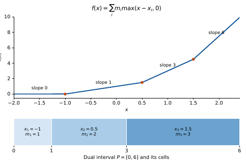
For a lattice polytope associated with an ample toric line bundle, the bounded convex functions constructed above correspond to continuous semipositive toric metrics. Their non-Archimedean Chern measures are obtained by the tropical comparison theorem, with the factor and the canonical section of tropicalization retained. The inverse construction on does not assert that an arbitrary measure on the entire analytic toric variety is determined by its tropical pushforward. The canonical invariant class and its section are part of the comparison.
References. This is a finite-dimensional proof of the compact-support case of the convex existence theorem used in [BGJK25] (Theorem 6.2.13 and Appendix A). The general theorem, its uniqueness, and its applications to toric metrics are treated there; the convex/metric dictionary is [GH] (Theorem 2.5.8). The minimization argument combines the Legendre correspondence with the volumes of the cells , and is included as a proof reconstruction rather than as a new existence result.
21.28 Toric metrics on subvarieties: the local weighted germ
A measure pushed to a tropical image does not by itself remember which analytic branch supplied its mass. This issue occurs both for subvarieties of abelian varieties and for subvarieties of toric varieties. It becomes essential when tropicalization is finite-to-one rather than injective.
The abelian case
In Gubler–Stadlöder’s setting over an algebraically closed complete nontrivially valued field, Raynaud uniformization provides a lattice , a real vector space , and affine cocycle functions . Continuous toric metrics on a line bundle correspond to continuous functions satisfying When is ample, convexity of is equivalent to semipositivity of the metric. Their approximation theorem preserves this cocycle; ordinary convolution or an arbitrary polyhedral approximation without the cocycle would not define a metric on the quotient. For a closed subvariety , the support of the canonical measure is independent of the chosen ample , and its map to the tropicalization is piecewise linear, surjective and finite-to-one. The measure formula on a polytopal decomposition of has multiplicities depending on , and the face, but not on the chosen toric metric. The canonical metric gives a sum of Lebesgue measures on those faces. This statement does not say that all faces have dimension or that all weights are one. The real Monge–Ampère measure on each face uses the affine space and normalization specified in that formula.
References. [GS23] (Theorems 1.1–1.3, Proposition 3.8 and Corollary 1.4).
The toric-subvariety comparison
Lin considers a subvariety of a toric variety over an algebraically closed complete nontrivially valued field. Put , and restrict to the torus locus. At a point of the tropical skeleton, the relevant object is the weighted tropicalization of the analytic germ at . A sufficiently small neighbourhood gives a representative of that germ. For a semipositive toric metric with tropical Green function , Theorem A of [Lin26] gives On an open face of dimension , the corresponding formula reduces to , transported by the face chart. Here the real measure is normalized by the face lattice and is its tropical weight. On lower-dimensional faces the full weighted neighbourhood is generally needed. Restricting to that face and taking its intrinsic real Hessian can lose transverse intersection mass.
Example 21.28.1. (Why a zero-dimensional restriction loses curvature). On , let . Its restriction to the face is the constant zero function. Nevertheless . The mass is the difference of the slopes on the two adjacent rays; it cannot be recovered from the value of the restricted function. This elementary example explains the need for a weighted germ. It is not a substitute for the higher-dimensional comparison theorem.
NAG-900445 Proof review pending
Lemma 21.28.2. (Pushforward does not identify branches). If a map has distinct points with , then equality of pushforward measures under does not imply equality of measures on .
Proof. The distinct measures and have the same pushforward. ◻
Consequently a tropical equality becomes an analytic equality only after one has supplied a support theorem, branchwise local formulas, or a sufficiently faithful family of maps with compatible measures. The strong faithfulness and absolute continuity assumptions in Section 16.8 are one specific way of obtaining this control. They should not be suppressed when applying a tropical solution to an analytic equation.
References. [Lin26] (Theorem A, Corollary B and Remark 9.8); the two elementary examples above isolate the information lost by restriction or pushforward.